
How Do Computers Come into the Art of Solving Puzzles? #PID1.4
Throughout history, puzzles have intrigued the human mind, not merely for entertainment but for the challenge they pose to logic, creativity, and persistence. From ancient labyrinths to Sudoku and the Rubik’s Cube, solving a puzzle often feels like an art — but beneath that art lies a surprising amount of structure. And where there is structure, computers can often outperform intuition.
At their core, puzzles are problems with constraints, and solving them requires a systematic approach to navigating possibilities. This is precisely the realm where computers shine. Unlike humans, computers are not limited by short-term memory, fatigue, or bias. They can execute algorithms tirelessly, evaluate vast search spaces, and spot patterns at a scale impossible for the human brain. As a result, computers don’t just mimic human puzzle-solving — they fundamentally transform it.
Why the Rubik’s Cube?
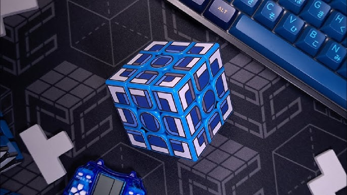
Among all puzzles, the Rubik’s Cube has emerged as a particularly fascinating object of study in computer science, mathematics, and algorithm design. Invented in 1974 by Ernő Rubik, it has over 43 quintillion unique configurations (43,252,003,274,489,856,000 to be exact). That’s more than the number of grains of sand on Earth or seconds since the Big Bang. And yet, with the right approach, any configuration can be solved in 20 moves or fewer — a result known as God’s Number.
But how does one go from a jumbled cube to the solution in such a short number of moves, especially when the total number of configurations is so massive?
This is where the mathematical beauty of the cube comes into play.
The Mathematics Behind the Cube
To a computer scientist or a mathematician, the Rubik’s Cube is more than just a toy — it’s a group. In group theory (a branch of abstract algebra), we define a group as a set with an operation that satisfies certain axioms: closure, associativity, identity, and inverses. Each move you make on a Rubik’s Cube — whether it’s a quarter-turn of a face or a full rotation — corresponds to an operation in this group.
The entire set of all possible cube states forms a permutation group. More specifically, it’s a subgroup of the symmetric group on the cube’s stickers, where each legal operation is a permutation of the cube’s pieces. The solved state is the group’s identity element, and solving the cube is equivalent to finding the inverse sequence of moves that returns any configuration to this identity.
From a computational perspective, this means that solving the cube becomes a path-finding problem in a highly structured space. The “nodes” are the cube states, and the “edges” are the moves that transform one state into another.
But this graph of states is unimaginably vast — far too large for brute force to be practical. Even if a computer could check a billion configurations per second, it would still take centuries to exhaustively search all 43 quintillion. Clearly, we need something smarter.
Why Brute Force Fails — and Algorithms Succeed
Imagine trying to solve the cube purely by random moves — it would be virtually impossible to land on the solved state, even in a lifetime. Even a depth-limited brute-force search, where the computer tries all sequences up to, say, 20 moves, quickly becomes intractable. At 18 legal face turns per move and 20 moves deep, that’s 18²⁰ ≈ 10²⁵ possibilities — still far beyond what any computer can handle.
That’s why we need algorithms. Algorithms introduce structure, allowing us to prune the search space intelligently. They leverage mathematical symmetries, identify key cube properties (like orientation, permutation, and parity), and break the problem into smaller, tractable sub-problems.
Rather than treating all configurations as equal, a good algorithm guides the computer through the space more like a mountaineer scaling peaks via well-worn trails rather than hacking blindly through a jungle.
What Computers Bring to Puzzle Solving
So why are computers particularly well-suited to this domain?
- Speed: Computers can simulate millions of cube manipulations per second.
- Memory: They can store large lookup tables — precomputed solutions to subproblems.
- Exhaustiveness: They don’t get bored or distracted; they follow through every branch of a search tree.
- Precision: No errors, no forgetfulness. Every move is logical, every decision traceable.
These strengths allow computers not only to solve the Rubik’s Cube but to solve it optimally — finding the shortest or most efficient solution using algorithmic planning.
From Human Intuition to Mathematical Algorithms
Before computers entered the scene, cube-solving was based largely on heuristics — trial-and-error, memorized sequences, and intuition. Speedcubers developed methods that worked well in practice but didn’t guarantee minimal solutions. It was the introduction of mathematical algorithms that changed the landscape.
The first major breakthrough came in the form of Thistlethwaite’s algorithm in the 1980s. It introduced the idea of reducing the cube’s complexity gradually by defining nested subgroups. From there, even more optimized approaches like Kociemba’s algorithm emerged, leveraging symmetries and lookup tables to reduce average solutions to around 20 moves.
Each of these algorithms doesn’t just find a solution — they exploit the cube’s algebraic structure to find efficient, systematic paths through its vast configuration space.
Thistlethwaite’s Algorithm – From Chaos to Structure
By the early 1980s, the Rubik’s Cube had become a global phenomenon — and a challenge that captivated not only hobbyists but also mathematicians. One such mind was Morwen Thistlethwaite, a mathematician who, in 1981, proposed one of the first major algorithmic breakthroughs in cube solving. His approach laid the foundation for many of the advanced solvers used today — not by brute force, but by applying the elegant machinery of group theory.
At its core, Thistlethwaite’s method turns the Rubik’s Cube into a layered mathematical structure — reducing the problem not in one step, but through a sequence of increasingly constrained subproblems. Each stage progressively shrinks the space of possible cube states, leveraging nested subgroups to transform an otherwise intractable problem into one that can be solved efficiently.
Modeling the Cube as a Group
To understand Thistlethwaite’s insight, we first need to recognize how the cube operates in algebraic terms.
Every legal move on a Rubik’s Cube can be considered a group generator — a function that permutes the pieces of the cube. The entire collection of these permutations forms a group G under function composition. This group is known as the Rubik’s Cube group, and it contains all 43 quintillion possible cube states.
Mathematically, a group (G) can be described by a presentation — a set of generators (moves) and relations (how these moves interact). In the cube’s case, common generators might include:
- (U): rotate the upper face 90° clockwise
- (R): rotate the right face 90° clockwise
- (F): front face, and so on
From just these generators and their inverses, all cube states can be reached.
The Key Insight: Subgroup Reduction
Thistlethwaite’s key insight was to partition the problem of solving the cube into a sequence of four nested subgroups:
$$ G_0 \supset G_1 \supset G_2 \supset G_3 \supset G_4 = { I } $$
Where:
- (G_0): the full cube group (all states)
- (G_1): subgroup where edge orientations are correct
- (G_2): subgroup where corners are also oriented
- (G_3): subgroup where all pieces are in correct slice layers
- (G_4): the identity group — the solved state
Each subgroup (G_{i+1}) is a proper subgroup of (G_i), meaning it contains fewer states, but is still closed under certain restricted moves.
For example:
- To move from (G_0)to (G_1), we only use moves that don’t disturb solved edge orientations.
- From (G_1) to (G_2), we constrain the move set further to preserve both edge and corner orientations.
By progressing through these subgroups, the algorithm ensures that with each phase, the cube becomes increasingly constrained — gradually forcing it into a state where the solution becomes trivial.
Phase-by-Phase Breakdown
Let’s briefly outline the four phases of Thistlethwaite’s algorithm:
Phase 1: Reduction to (G_1)
Objective: Correct the orientation of all 12 edges.
- Move set allowed: all face turns
- Edge orientation is a binary invariant (flipped or not)
- The space of states reduces from ~(4.3 \times 10^{19}) to about (10^9)
Phase 2: Reduction to (G_2)
Objective: Correct the orientation of corners and place all edges in their correct slice layers (middle or outer).
- Move set restricted to half-turns on some faces (e.g., only U, D, R2, L2, F2, B2)
- Corner orientation: 3 values per corner (0°, 120°, 240°)
- State space drops to ~(10^7)
Phase 3: Reduction to (G_3)
Objective: Place all pieces (edges and corners) in their correct orbits (positions relative to centers).
- Only even permutations are allowed
- Reduction to ~(10^5) possible states
Phase 4: Solve the cube (from (G_3) to identity)
Objective: Use only the remaining allowed moves to reach the solved state.
At each stage, Thistlethwaite’s method restricts the move set, guiding the cube closer to a structured state while simultaneously reducing the number of legal transformations — and therefore the size of the search space.
Why It Works: Mathematics Meets Efficiency
This hierarchical decomposition is more than a clever trick. It relies on coset decomposition from group theory. If we think of the Rubik’s Cube group (G) as a forest of interconnected trees, Thistlethwaite’s method picks one “layer” of branches at a time, cutting off all but the ones that eventually lead to the root (solved state). This avoids wandering aimlessly through the forest and allows for guided, phase-wise convergence.
Another advantage is modularity. Since each phase has a much smaller state space, it becomes feasible to precompute lookup tables (called pruning tables) for each subgroup. These tables store the shortest number of moves needed to reach the next subgroup from any configuration in the current one — dramatically reducing computation time during solving.
Conclusion
Although Thistlethwaite’s algorithm does not always find the absolute shortest solution (i.e., not always “God’s Algorithm”), it typically solves any scrambled cube in 45 to 52 moves — a remarkable feat considering the cube’s astronomical complexity.
Thistlethwaite’s algorithm laid the groundwork for efficient Rubik’s Cube solving by breaking down the problem into manageable phases — next, we’ll explore how Kociemba’s algorithm builds on this foundation to achieve even faster and shorter solutions.
Related Posts
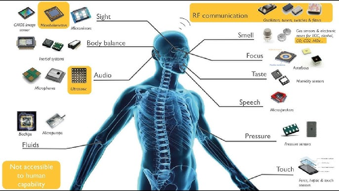
Sensors in Robotics: How Ultrasonic, LiDAR, and IMU Work
Sensors are to robots what eyes, ears, and skin are to humans—but with far fewer limits. While we rely on just five senses, robots can be equipped with many more, sensing distances, movement, vibrations, orientation, light intensity, and even chemical properties. These sensors form the bridge between the digital intelligence of a robot and the physical world it operates in.
Read more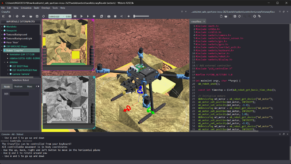
Debugging a Robot In Simulation Before You Burn Wires
Hardware does not come with an undo button. Once you power it on, mistakes—from reversed wiring to faulty code—can result in costly damage. Motors may overheat, printed circuit boards (PCBs) can be fried, and sensors may break. These issues turn exciting projects into frustrating repair sessions. The autonomous drone shown above, designed for GNSS-denied environments in webots as part of the ISRO Robotics Challenge, is a perfect example—where careful planning, testing, and hardware safety were critical at every step
Read more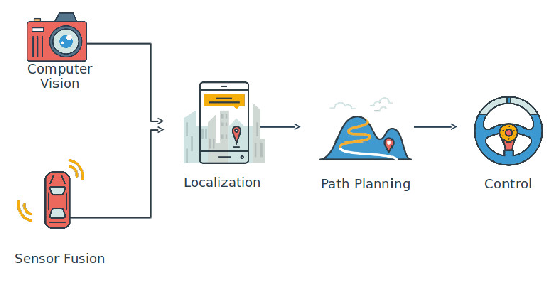
Computer Vision vs. Sensor Fusion: Who Wins the Self-Driving Car Race?
Tesla’s bold claim that “humans drive with eyes and a brain, so our cars will too” sparked one of the most polarizing debates in autonomous vehicle (AV) technology: Can vision-only systems truly compete with—or even outperform—multi-sensor fusion architectures?
Read more