
Kociemba’s Algorithm – The Two-Phase Breakthrough #PID1.5
Kociemba’s algorithm revolutionizes Rubik’s Cube solving by efficiently navigating the immense complexity of the cube’s state space using advanced mathematical tools from group theory and heuristic search. This two-phase method strikes a balance between tractability and optimality, making it a cornerstone of computational puzzle solving.
The Mathematical Setup: Group Theory and Cosets
Recall that the Rubik’s Cube group (G) consists of all legal cube states under composition of moves. Kociemba’s method strategically divides (G) into cosets of a carefully chosen subgroup (H \subseteq G):
$$ G = \bigcup_{g \in G/H} gH $$
Here, (H) is the subgroup of cube states where all edges and corners are oriented correctly and all middle slice edges are located within the middle layer. This subgroup is sometimes called the “half-turn metric group”, since allowed moves in (H) correspond to half-turns of certain faces.
By reducing the problem to first finding the coset representative (g) that brings the cube into (H) (Phase 1), and then solving within (H) (Phase 2), the algorithm exploits the quotient structure (G/H) to manage complexity.
Phase 1: Reducing to the Subgroup (H)
Phase 1’s goal is to transform any scrambled cube state (s \in G) into a state (s’ \in H) . Formally, find a sequence of moves (m_1) such that:
$$ s’ = m_1 \cdot s \in H $$
Where (m_1) is a product of face turns (quarter or half turns).
- Edge orientation: Each edge can be in two states — oriented or flipped — giving a binary invariant. There are (2^{12} = 4096) possible edge orientation states.
- Corner orientation: Each corner can be oriented in 3 ways, so (3^8 = 6561) corner orientations.
- Middle slice edges: The position of the four middle-layer edges is constrained.
All these constraints define (H) , which contains approximately (10^{10}) states.
Phase 1’s problem reduces to finding a minimal-length (m_1) to reach (H) , which is a constrained subgroup problem in the Rubik’s cube group.
Phase 2: Solving within (H)
Once the cube is in (H) , Phase 2 searches for a move sequence (m_2) restricted to moves within (H) such that:
$$ m_2 \cdot s’ = I $$
where (I) is the solved state.
Since moves in (H) preserve edge and corner orientation and slice position, the search space is drastically smaller than the full (G) .
Heuristics and Pattern Databases: Guiding the Search
Direct brute-force search over (G) or even (H) is impossible due to the astronomical number of states. To tackle this, Kociemba’s algorithm employs heuristic search algorithms — specifically, Iterative Deepening A* (IDA*) — powered by pattern databases (PDBs).
What are Pattern Databases?
PDBs are precomputed lookup tables storing the exact minimal number of moves required to solve specific cube features, such as edge orientation or corner permutation, ignoring other features.
For example, one PDB might store the minimal moves to solve edge orientation, regardless of corner orientation or permutation.
Since these databases cover disjoint subsets of the cube’s state, their heuristic values can be combined by taking the maximum to ensure admissibility (never overestimating).
This maximum value guides IDA* to explore only states promising to be close to the solution, pruning vast regions of the search space.
IDA* Search Algorithm
IDA* is a memory-efficient variant of A* that performs depth-first searches with increasing cost thresholds.
At each iteration:
The search depth limit is set by the heuristic cost (f = g + h) , where:
- (g) = cost from start to current node (number of moves so far)
- (h) = heuristic estimate of moves to goal (from PDB)
The algorithm explores all nodes with (f \leq) threshold.
If no solution found, threshold increases, and search repeats.
IDA*’s use in Kociemba’s algorithm ensures that:
- The first solution found is guaranteed to be minimal within the move restrictions.
- Memory overhead remains manageable, even for large state spaces.
Formalizing the Heuristic Function
If we define heuristic functions:
- (h_{EO}(s)): minimal moves to solve edge orientation in state (s)
- (h_{CO}(s)): minimal moves to solve corner orientation
- (h_{EP}(s)): minimal moves to place edges in their correct slices
- (h_{CP}(s)): minimal moves to permute corners correctly
Then the combined heuristic (h(s)) guiding the search is:
$$ h(s) = \max { h_{EO}(s), h_{CO}(s), h_{EP}(s), h_{CP}(s) } $$
This ensures the search never expands nodes that cannot lead to an optimal solution.
Summary of the Mathematical Power
Kociemba’s algorithm elegantly balances:
- Algebraic structure: Using subgroup and coset decompositions to reduce complexity
- Heuristic efficiency: Pattern databases provide admissible heuristics guiding the search
- Search algorithm: IDA* ensures optimal paths under given constraints
This synergy enables the solver to consistently find solutions averaging around 20 moves (half the move length of Thistlethwaite’s original algorithm) in milliseconds on modern computers — a feat that would be impossible without this deep mathematical foundation.
Other Algorithms: A Brief Overview and Comparison
While Kociemba’s algorithm is among the most widely used for computational Rubik’s Cube solving due to its efficiency and near-optimal solutions, it is part of a broader landscape of methods, each with its own mathematical basis, advantages, and limitations.
Thistlethwaite’s Algorithm Revisited
As discussed earlier, Thistlethwaite’s algorithm partitions the cube group into a sequence of four nested subgroups:
$$ G = G_0 \supset G_1 \supset G_2 \supset G_3 \supset G_4 = { I } $$
By solving the cube progressively through these subgroups, it guarantees a solution in at most 52 moves (in half-turn metric). While theoretically elegant, the multiple phases and larger intermediate state spaces make it computationally heavier compared to Kociemba’s two-phase approach.
God’s Algorithm
God’s Algorithm is the theoretical ideal that always finds the shortest possible solution for any cube position. It relies on exhaustive search of the entire state space ((\approx 4.3 \times 10^{19}) states) using massive computational resources and precomputed tables, such as the famous Table of 20 moves or less (God’s Number = 20).
While this guarantees the absolute shortest solution, it is impractical for general use due to storage and computation demands. Kociemba’s algorithm often approximates God’s Algorithm efficiently by using heuristics and subgroup constraints.
CFOP (Fridrich Method)
On the practical speedcubing side, CFOP (Cross, F2L, OLL, PLL) is a human method rather than a computer algorithm. It relies on heuristic algorithms and pattern recognition rather than exhaustive search or mathematical group theory. While CFOP solves the cube very fast for humans, its move counts tend to be longer and less optimized compared to computational methods like Kociemba’s.
Other Computational Approaches
- Korf’s Algorithm: Utilizes IDA* with large pattern databases for optimal solutions but is computationally expensive.
- Macro-Operators and Pruning Tables: Many solvers employ precomputed tables for specific cube configurations or use machine learning to predict move sequences.
- Genetic Algorithms and AI: Recent work explores reinforcement learning and evolutionary strategies to solve cubes without explicit group theory, focusing on policy learning and move prediction.
Comparison Summary
| Algorithm | Move Optimality | Computational Complexity | Use Case |
|---|---|---|---|
| God’s Algorithm | Guaranteed minimal | Very high | Theoretical, research |
| Kociemba’s Algorithm | Near-optimal (~20 moves) | Moderate | Fast, practical solvers |
| Thistlethwaite’s | Moderate (~52 moves max) | Higher | Theoretical, educational |
| CFOP | Longer (~50+ moves) | Low | Human speedcubing |
| Korf’s Algorithm | Optimal | Very high | Small subsets or specific puzzles |
Final Thoughts
The mathematical sophistication of Rubik’s Cube algorithms reveals how computers transform the art of puzzle-solving. From the elegant subgroup decompositions of Thistlethwaite and Kociemba to heuristic-guided searches, computers convert what once was a purely human trial-and-error activity into a rigorous, near-optimal science.
Understanding these algorithms highlights the power of:
- Algebraic abstractions (groups, cosets) to simplify complex states
- Heuristic functions to efficiently guide searches
- Iterative search algorithms that balance time and space constraints
In the next post, we will delve deeper into practical implementations of Kociemba’s algorithm and how modern solvers leverage these concepts to provide instant solutions.
Related Posts
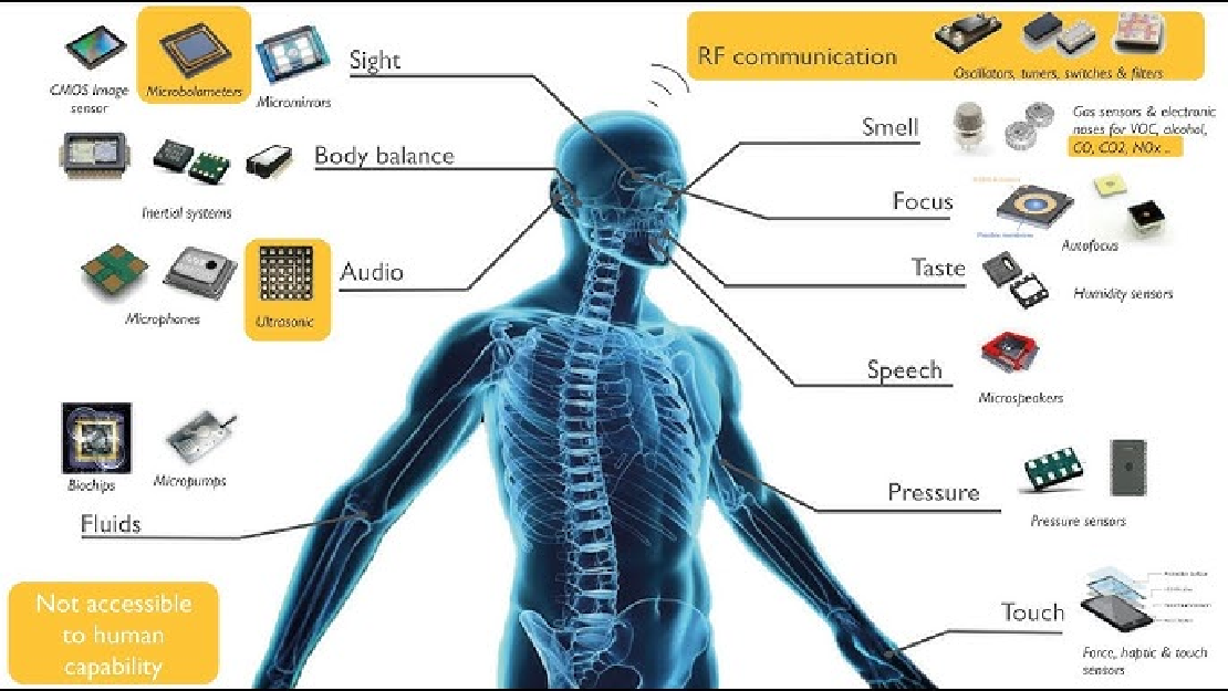
Sensors in Robotics: How Ultrasonic, LiDAR, and IMU Work
Sensors are to robots what eyes, ears, and skin are to humans—but with far fewer limits. While we rely on just five senses, robots can be equipped with many more, sensing distances, movement, vibrations, orientation, light intensity, and even chemical properties. These sensors form the bridge between the digital intelligence of a robot and the physical world it operates in.
Read more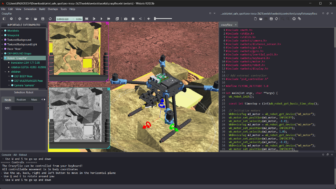
Debugging a Robot In Simulation Before You Burn Wires
Hardware does not come with an undo button. Once you power it on, mistakes—from reversed wiring to faulty code—can result in costly damage. Motors may overheat, printed circuit boards (PCBs) can be fried, and sensors may break. These issues turn exciting projects into frustrating repair sessions. The autonomous drone shown above, designed for GNSS-denied environments in webots as part of the ISRO Robotics Challenge, is a perfect example—where careful planning, testing, and hardware safety were critical at every step
Read more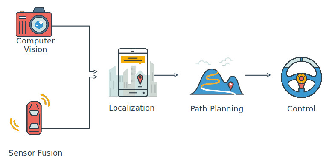
Computer Vision vs. Sensor Fusion: Who Wins the Self-Driving Car Race?
Tesla’s bold claim that “humans drive with eyes and a brain, so our cars will too” sparked one of the most polarizing debates in autonomous vehicle (AV) technology: Can vision-only systems truly compete with—or even outperform—multi-sensor fusion architectures?
Read more