
The Mathematics Behind the Rubik’s Cube #PID1.3
The Rubik’s Cube is not just a puzzle; it’s a deep mathematical object grounded in group theory, combinatorics, and geometry. Understanding the math behind it allows us to grasp why it has 43 quintillion possible states, how we categorize moves, and why some solutions are more efficient than others.
Group Theory and the Rubik’s Cube
Group theory is a branch of mathematics that studies sets with operations that follow specific rules. The Rubik’s Cube can be seen as a mathematical group where:
- Each state of the cube is an element of the group.
- Each valid move (rotating a face) is a group operation.
- The identity element is the solved state of the cube.
- Moves have inverses (e.g., turning the right face clockwise can be undone by turning it counterclockwise).
The Rubik’s Cube belongs to a finite group since it has a limited number of positions. The set of all possible cube configurations, with the operation of applying a sequence of moves, forms a non-abelian group (meaning that order matters—doing move A then B is not the same as doing move B then A).
Here’s the updated version incorporating center orientation in the usual order for 3×3 scales:
Order of an Element in the Rubik’s Cube Group
In group theory, the order of an element is the number of times it must be applied to return to the identity (solved state). In the Rubik’s Cube, certain moves or sequences have different orders:
- A single quarter-turn of a face has order 4 (doing it four times returns the cube to the original state).
- A 180-degree turn has order 2.
- Certain complex sequences have higher orders, meaning they take more repetitions to cycle back to the starting position.
- On a standard 3×3 Rubik’s Cube, center pieces do not change position, but their orientation can matter in some cases, such as in supercube variants where sticker orientation is tracked. In such cases, center rotations may introduce elements of order 2 or 4, depending on the move sequence.
Understanding the order of moves, including center orientation, helps in designing efficient solving algorithms.
Counting the 43 Quintillion Permutations
To compute the number of possible Rubik’s Cube states, we analyze the degrees of freedom:
- There are 8 corner pieces, each of which can be arranged in (8!) ways.
- Each corner has three orientations, giving (3^7) possibilities (the last one is determined by the others).
- There are 12 edge pieces, which can be arranged in (12!) ways.
- Each edge has two orientations, giving (2^{11}) possibilities (the last one is determined by the others).
- However, only even permutations of corners and edges are possible, so we divide by 2.
Thus, the total number of possible Rubik’s Cube states is:
$$ \frac{8! \times 3^7 \times 12! \times 2^{11}}{2} = 43,252,003,274,489,856,000 $$
which is approximately 43 quintillion.
For the 2×2×2 Rubik’s Cube, we use a similar method but without considering edges:
- The 8 corner pieces can be arranged in (8!) ways.
- Each has 3 orientations, giving (3^7) (since the last one is determined).
- Only even permutations are possible, so we divide by 2.
Thus, the number of possible 2×2×2 states is:
$$ \frac{8! \times 3^7}{2} = 3,674,160 $$
which is significantly smaller than the 3×3×3 but still quite large.
God’s Number and Move Metrics
God’s Number is the maximum number of moves required to solve the worst-case scenario of a Rubik’s Cube optimally. In 2010, researchers proved that God’s Number for a standard 3×3×3 Rubik’s Cube is 20 moves in the quarter-turn metric (where each 90-degree face turn counts as one move).
Move Metrics
- Quarter-Turn Metric (QTM): Every 90-degree turn is counted as one move. This is the standard used in the 20-move God’s Number proof.
- Half-Turn Metric (HTM): Both 90-degree and 180-degree turns count as one move. In this metric, God’s Number is 18 moves.
- Face-Turn Metric (FTM): Any rotation of a face, whether 90, 180, or 270 degrees, is counted as one move.
Different solving methods optimize for different metrics. For example, speedcubers prioritize fewer moves in practice rather than the theoretical minimum number of moves.
Euclidean and Quaternion Mathematics in the Rubik’s Cube
Euclidean Geometry and the Rubik’s Cube
The Rubik’s Cube exists in three-dimensional Euclidean space, meaning its transformations can be represented using classical geometric tools such as matrices and vector operations.
Rotation Matrices: Each face rotation can be described using a 3×3 rotation matrix. A 90-degree clockwise rotation about the x, y, or z-axis can be represented as:
$$ R_x(90^\circ) = \begin{bmatrix} 1 & 0 & 0 \ 0 & 0 & -1 \ 0 & 1 & 0 \end{bmatrix}, $$
$$ R_y(90^\circ) = \begin{bmatrix} 0 & 0 & 1 \ 0 & 1 & 0 \ -1 & 0 & 0 \end{bmatrix}, $$
$$ R_z(90^\circ) = \begin{bmatrix} 0 & -1 & 0 \ 1 & 0 & 0 \ 0 & 0 & 1 \end{bmatrix}. $$
Vector Representation: Each cubie (small cube piece) has a position vector ( v ), and applying a rotation matrix transforms it to a new position: $$ v’ = R v. $$ Using these transformations, all possible moves on the cube can be described mathematically.
Quaternion Representation and the Rubik’s Cube
Quaternions offer an alternative way to describe rotations in 3D space. A quaternion is defined as: $$ q = a + bi + cj + dk, $$ where ( a, b, c, d ) are real numbers, and ( i, j, k ) are imaginary unit vectors satisfying specific multiplication rules.
Rotation Using Quaternions: Any 3D rotation can be represented as: $$ q = \cos\left(\frac{\theta}{2}\right) + \sin\left(\frac{\theta}{2}\right)(xi + yj + zk), $$ where ( \theta ) is the rotation angle, and ( (x, y, z) ) is the rotation axis.
Applying a Rotation: Given a point represented by a quaternion ( p ), the rotated point ( p’ ) is obtained as: $$ p’ = q p q^{-1}. $$
Using quaternions avoids issues like gimbal lock and allows smooth, efficient calculations, making them useful in robotic cube solvers and computer simulations.
Comparison of Euclidean and Quaternion Methods
| Method | Advantages | Use Case in Rubik’s Cube |
|---|---|---|
| Rotation Matrices | Simple, easy to compute | Manual cube manipulation, algebraic solving |
| Quaternions | No gimbal lock, computationally efficient | Robotics, computer simulations |
While human solvers primarily use group-theoretic approaches, understanding Euclidean and quaternion mathematics is valuable for computational methods and AI-driven solutions.
Advanced Mathematics Behind the Rubik’s Cube
Graph Theory and the Rubik’s Cube
The entire state space of the Rubik’s Cube can be visualized as a graph, where:
- Each node represents a unique cube configuration.
- Each edge represents a valid move between two configurations.
This allows us to analyze cube solving as a shortest path problem (like in Dijkstra’s algorithm). The challenge is that this graph is huge, containing about 43 quintillion nodes! Researchers have used Breadth-First Search (BFS) to explore how quickly the cube can be solved from any state, leading to the proof of God’s Number (20 in QTM).
Markov Chains and Random Scrambles
If you randomly twist a Rubik’s Cube, how many moves does it take before it is “fully scrambled”? This is a classic Markov Chain problem, where each move represents a random transition between states. Studies suggest that after about 19-20 random moves, the cube is statistically close to a uniformly random state. This insight is used in competitive cubing to ensure fairness in official scramble generation.
Group Structure: Conjugacy Classes and Commutators
The Rubik’s Cube group has special elements called commutators and conjugates, which are fundamental to advanced solving techniques:
- Commutator: ([A, B] = A B A^{-1} B^{-1}) – used in many algorithms to isolate cube pieces.
- Conjugate: (X A X^{-1}) – applies a transformation in a different context.
These concepts allow cube solvers to move a small set of pieces without disrupting the rest, forming the basis for algorithms like CFOP, Roux, and ZZ methods.
Why Is Solving the Cube Hard? Computational Complexity
Solving an arbitrary cube position optimally (in the least moves) is an NP-hard problem. That means there is no known efficient algorithm that can solve every case optimally in polynomial time. This is why human solvers use heuristic-based approaches like CFOP, Petrus, and Roux, rather than brute force computation.
What’s Next? Computers and Efficient Cube Solving
In our next post, we will explore how computers approach solving the Rubik’s Cube, including AI techniques, heuristics, and optimal solvers like Kociemba’s Algorithm and DeepCubeA.
Related Posts
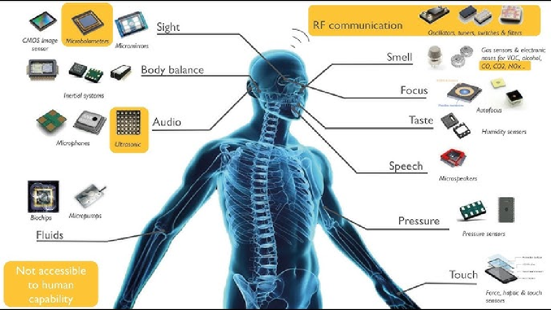
Sensors in Robotics: How Ultrasonic, LiDAR, and IMU Work
Sensors are to robots what eyes, ears, and skin are to humans—but with far fewer limits. While we rely on just five senses, robots can be equipped with many more, sensing distances, movement, vibrations, orientation, light intensity, and even chemical properties. These sensors form the bridge between the digital intelligence of a robot and the physical world it operates in.
Read more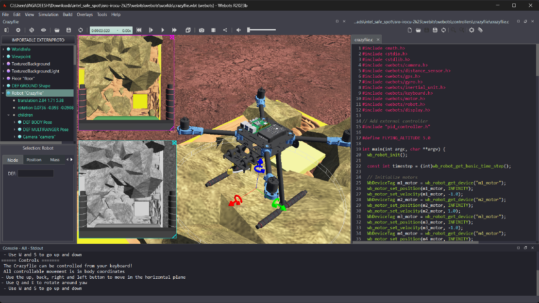
Debugging a Robot In Simulation Before You Burn Wires
Hardware does not come with an undo button. Once you power it on, mistakes—from reversed wiring to faulty code—can result in costly damage. Motors may overheat, printed circuit boards (PCBs) can be fried, and sensors may break. These issues turn exciting projects into frustrating repair sessions. The autonomous drone shown above, designed for GNSS-denied environments in webots as part of the ISRO Robotics Challenge, is a perfect example—where careful planning, testing, and hardware safety were critical at every step
Read more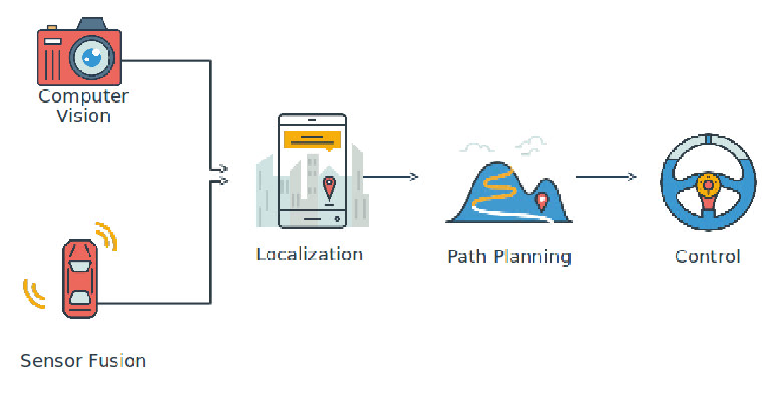
Computer Vision vs. Sensor Fusion: Who Wins the Self-Driving Car Race?
Tesla’s bold claim that “humans drive with eyes and a brain, so our cars will too” sparked one of the most polarizing debates in autonomous vehicle (AV) technology: Can vision-only systems truly compete with—or even outperform—multi-sensor fusion architectures?
Read more