
What is SLAM? And Why It’s the Brain of Mobile Robots
- #Slam
- #Simultaneous Localization and Mapping
- #Robotics
- #Mobile Robots
- #Mapping
- #Localization
- #Sensors
- #Lidar
- #Computer Vision
- #Probabilistic Robotics
- #Kalman Filter
- #Particle Filter
- #Robot Navigation
- #Autonomous Systems
- #Path Planning
- #3d Mapping
- #Robotics Perception
- #Sensor Fusion
- #Robotics Algorithms
- #Robotics Software
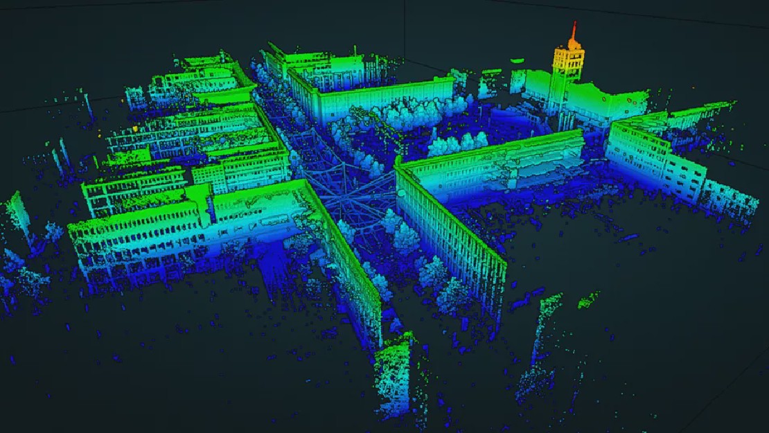
In robotics, SLAM—Simultaneous Localization and Mapping—is regarded as one of the most fundamental and complex problems. At its core, SLAM addresses a deceptively simple question: “Where am I, and what does the world around me look like?”
For a robot to navigate autonomously, it must construct a map of an unknown environment while simultaneously localizing itself within that map. This dual-estimation problem underpins most mobile robotics systems, making SLAM essentially the cognitive core or brain that enables autonomy.
The Formal Problem Definition
The SLAM problem can be formally expressed in probabilistic terms. Let:
- xₜ denote the robot’s state (pose) at time t.
- m represent the map of the environment (which may be feature-based, occupancy grid, or landmark-based).
- uₜ be the control input (e.g., wheel velocity commands).
- zₜ be the observation or sensor measurement at time t.
The goal of SLAM is to compute the posterior distribution:
$$ P(x_{1:t}, m \mid z_{1:t}, u_{1:t}) $$
That is, we want to estimate the trajectory of the robot x₁:t and the map m, given all sensor observations z₁:t and control inputs u₁:t up to time t. This joint estimation makes SLAM non-trivial, since errors in one (pose or map) propagate into the other.
A Bayesian Perspective
The SLAM problem is inherently a Bayesian inference problem. The recursive Bayes filter provides the framework:
$$ P(x_t, m \mid z_{1:t}, u_{1:t}) = \eta \cdot P(z_t \mid x_t, m) \cdot \int P(x_t \mid x_{t-1}, u_t) P(x_{t-1}, m \mid z_{1:t-1}, u_{1:t-1}) dx_{t-1} $$
Where:
- \(\eta\) is a normalizing constant.
- \(P(z_t \mid x_t, m)\) is the observation model, also known as the likelihood.
- \(P(x_t \mid x_{t-1}, u_t)\) is the motion model, describing the robot’s kinematics.
This recursive structure is at the heart of many SLAM algorithms and leads to various implementations like Extended Kalman Filter SLAM, Particle Filter SLAM (FastSLAM), and Graph-Based SLAM.
State Estimation and Mapping
In SLAM, there are two intertwined estimation problems:
- Localization: Estimating the robot’s pose \(x_t\) given a map.
- Mapping: Estimating the map \(m\) given the pose history.
These are not independent—if the robot’s pose is uncertain, the resulting map will be too. This mutual dependency necessitates a joint estimation.
Motion Model
Assuming a differential drive robot, the motion model is often modeled as:
$$ x_t = f(x_{t-1}, u_t) + w_t $$
Where:
- \(f\) is the motion function (e.g., based on odometry).
- \(w_t\) is process noise, often modeled as zero-mean Gaussian noise with covariance \(Q_t\).
Observation Model
Sensor measurements (from LIDAR, sonar, or cameras) depend on the robot’s pose and the environment:
$$ z_t = h(x_t, m) + v_t $$
Where:
- \(h\) is the observation function.
- \(v_t\) is observation noise, modeled as Gaussian with covariance \(R_t\).
Variants and Algorithms
Depending on how one approximates the posterior, several algorithmic variants of SLAM arise:
Extended Kalman Filter SLAM (EKF-SLAM)
EKF-SLAM linearizes the motion and observation models around the current estimate and tracks the mean and covariance of the joint state \((x_t, m)\). It scales poorly with the number of landmarks due to quadratic complexity in the state size.
Particle Filter SLAM (FastSLAM)
FastSLAM uses a Rao-Blackwellized particle filter, factorizing the SLAM posterior:
$$ P(x_{1:t}, m \mid z_{1:t}, u_{1:t}) = P(m \mid x_{1:t}, z_{1:t}) \cdot P(x_{1:t} \mid z_{1:t}, u_{1:t}) $$
Particles represent different possible robot trajectories, and each particle maintains its own map, allowing for greater scalability and handling of non-linear, non-Gaussian systems.
Graph-Based SLAM
Graph SLAM formulates SLAM as a nonlinear optimization problem. Nodes in the graph represent robot poses and landmarks, while edges represent spatial constraints derived from motion and sensor data. The optimization seeks to find the configuration that minimizes the total error (e.g., via least-squares):
$$ x^* = \arg \min_x \sum_{i,j} | z_{ij} - h(x_i, x_j) |^2_{\Omega_{ij}} $$
Where \(\Omega_{ij}\) is the information matrix (inverse of the covariance).
Graph SLAM is currently one of the most popular SLAM formulations, especially in systems like g2o and Ceres Solver, due to its flexibility and ability to incorporate loop closures and global constraints.
The Role of SLAM in Mobile Robots
In the broader system architecture of a mobile robot, SLAM functions as the spatial intelligence unit. All downstream tasks—path planning, obstacle avoidance, exploration, and task execution—rely on accurate state and environment estimates.
SLAM enables:
- Real-time tracking of the robot’s pose.
- Dynamic updates to the map as new observations are made.
- Consistent correction of errors via loop closure detection.
- Integration with higher-level cognition systems like planning and decision-making.
Without SLAM, a mobile robot is effectively blind and disoriented—capable of sensing but not understanding its environment.
SLAM and Lie Groups
For robots operating in 2D or 3D, pose estimation involves dealing with SE(2) or SE(3) Lie groups. A pose is not just a vector but a transformation matrix involving rotation and translation:
$$ T = \begin{bmatrix} R & t \ 0 & 1 \end{bmatrix} \in SE(3) $$
Where:
- \(R \in SO(3)\) is a rotation matrix.
- \(t \in \mathbb{R}^3\) is a translation vector.
Modern SLAM back-ends incorporate these group structures to ensure consistency in optimization, using tools like manifold-aware optimization and Lie algebra exponential maps.
SLAM Beyond Geometry
While SLAM traditionally focuses on geometric mapping, there is increasing interest in semantic SLAM—embedding meaning and object-level understanding into the map. This blends SLAM with computer vision and deep learning, creating a more human-interpretable world model.
Final Thoughts
SLAM is not just a technique—it is the cognitive foundation of spatial intelligence in autonomous robots. It encapsulates estimation theory, probability, optimization, geometry, and control into a cohesive framework. As robotics systems grow more complex and dynamic, SLAM continues to evolve at the intersection of theory and real-world performance.
Whether using Kalman filters, particle filters, or factor graphs, SLAM remains the mathematical brain that allows robots to think spatially—bridging perception with action.
Related Posts
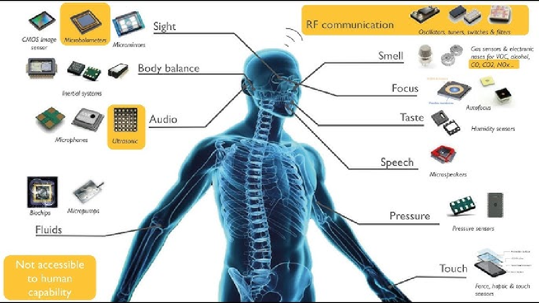
Sensors in Robotics: How Ultrasonic, LiDAR, and IMU Work
Sensors are to robots what eyes, ears, and skin are to humans—but with far fewer limits. While we rely on just five senses, robots can be equipped with many more, sensing distances, movement, vibrations, orientation, light intensity, and even chemical properties. These sensors form the bridge between the digital intelligence of a robot and the physical world it operates in.
Read more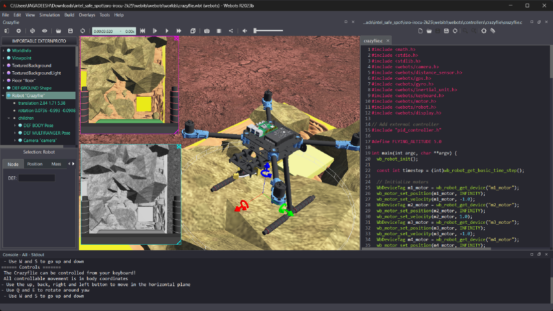
Debugging a Robot In Simulation Before You Burn Wires
Hardware does not come with an undo button. Once you power it on, mistakes—from reversed wiring to faulty code—can result in costly damage. Motors may overheat, printed circuit boards (PCBs) can be fried, and sensors may break. These issues turn exciting projects into frustrating repair sessions. The autonomous drone shown above, designed for GNSS-denied environments in webots as part of the ISRO Robotics Challenge, is a perfect example—where careful planning, testing, and hardware safety were critical at every step
Read more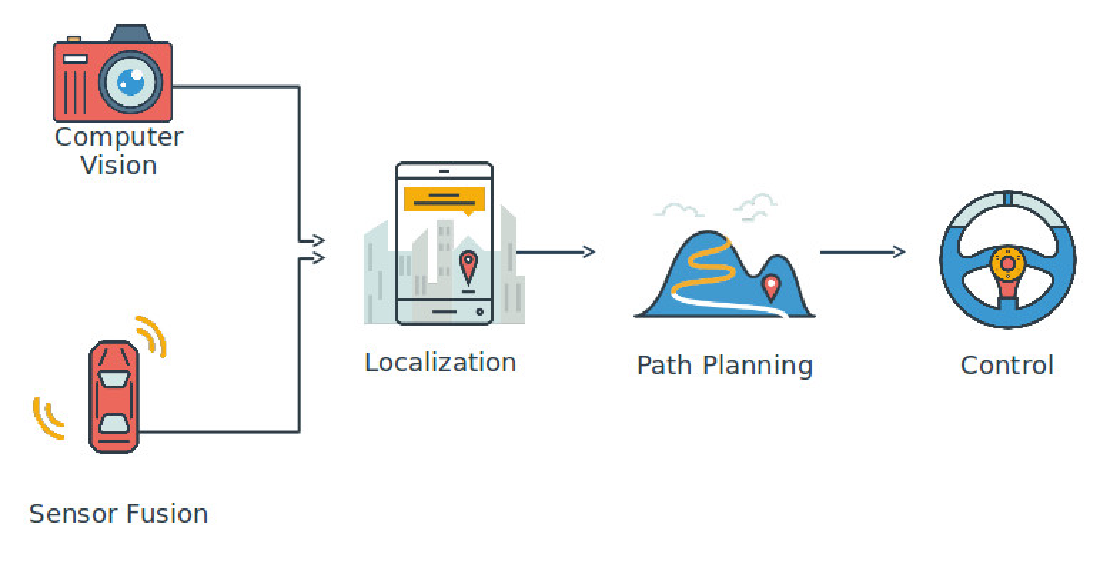
Computer Vision vs. Sensor Fusion: Who Wins the Self-Driving Car Race?
Tesla’s bold claim that “humans drive with eyes and a brain, so our cars will too” sparked one of the most polarizing debates in autonomous vehicle (AV) technology: Can vision-only systems truly compete with—or even outperform—multi-sensor fusion architectures?
Read more