Hardware Approaches to Floating-Point Transcendental Function Computation: CORDIC, PR-CORDIC, and LUT+Polynomial
Computing sin(x), cos(x), arctan(x), e^x, and ln(x) in hardware is not as obvious as it sounds. Software on a general-purpose CPU offloads these to a floating-point unit backed by microcode – the hardware is there, the problem has already been solved, and you call the function. On an FPGA or in a custom ASIC accelerator, none of that infrastructure exists. You have logic resources, DSP blocks if you are lucky, and the task of building a datapath that computes the right answer, with the right precision, at the right throughput, while fitting in the area you have.
This post covers the two dominant algorithmic families – CORDIC and LUT+Polynomial – along with their concrete implementations, the numerical structure that drives the design decisions, and where each approach actually wins on real hardware.
The Problem: Why Hardware Transcendental Functions Are Non-Trivial
The issue starts with what a floating-point number actually is. IEEE-754 single precision encodes a value as:
(-1)^S  x  1.mantissa  x  2^(exp - 127)

 [ S | Exponent (8 bits) | Mantissa (23 bits) ]
  1b        biased 127          implicit leading 1
The sign bit, an 8-bit biased exponent, and a 23-bit mantissa with an implicit leading 1. That gives representable values from roughly 1.2×10^-38 to 3.4×10^38.
This creates the first problem for any transcendental computation: the input range is enormous. sin(10^38) is a perfectly valid IEEE-754 input. Polynomial approximations only work well on small, bounded intervals. CORDIC needs a bounded angle to converge. Neither approach can handle the raw input range directly. Both require range reduction – a preprocessing step that uses periodicity, symmetry, and algebraic identities to map any valid input into a small canonical domain before the actual computation begins.
For sin and cos, the key identity is periodicity and quarter-wave symmetry: sin(x) is periodic with period 2π, and the behavior in [0, π/2] determines the behavior everywhere via sign and argument reflection. For e^x, the identity e^x = 2^(x/ln2) separates the integer and fractional parts of x/ln2, leaving only the fractional part (which is in [0, 1)) to evaluate. For ln(x), the IEEE-754 mantissa is already in [1, 2) by definition, which makes range reduction almost trivial – the exponent field directly gives the integer part of the logarithm.
| Function | Domain | Reduction method | Reduced domain |
|---|---|---|---|
| sin πx | (-2^128, 2^128) \ {0} | Periodicity + quadrant symmetry | [0, 0.5] |
| cos πx | (-2^128, 2^128) \ {0} | Periodicity + quadrant symmetry | [0, 0.5] |
| arctan(x)/π | (-2^128, 2^128) \ {0} | Identity arctan(x) + arctan(1/x) = π/2 | [0, 1] |
| e^x | [-126 ln2, 128 ln2) | e^x = 2^int · 2^frac | [0, 1) |
| ln(x) | [2^-126, 2^128) | Extract IEEE-754 exponent, mantissa in [1,2) | [1, 2) |
Range reduction precedes both CORDIC and polynomial evaluation. The difference between the approaches is what happens after reduction.
CORDIC: Coordinate Rotation DIgital Computer
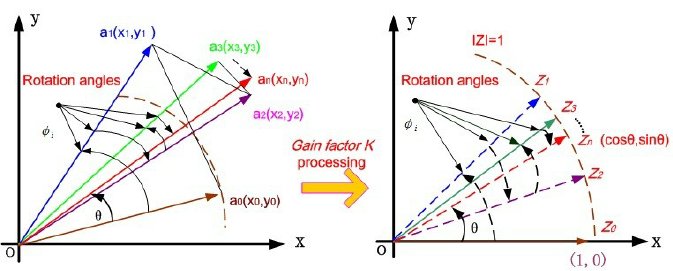
CORDIC was introduced by Jack Volder in 1959. The central insight is that rotating a 2D vector by an angle θ can be decomposed into a sequence of elementary rotations by precomputed angles, where each elementary rotation only requires a shift and an addition. No multipliers anywhere in the datapath.
The Rotation Decomposition
A standard 2D rotation by angle θ transforms (x, y) to:
x' = x cos(θ) - y sin(θ)
y' = y cos(θ) + x sin(θ)
This requires four multiplications and two additions, which is expensive. CORDIC avoids the multiplications by choosing θ cleverly. If the target angle is decomposed as a sum of elementary angles where each elementary angle is arctan(2^-i):
θ ≈ Σ  d_i · arctan(2^-i),    d_i ∈ {-1, +1}
    i=0
then the rotation by arctan(2^-i) has a scale factor of (1 + 2^-2i)^(1/2), and the actual rotation equations for that elementary step are:
x_{i+1} = x_i - d_i · 2^{-i} · y_i
y_{i+1} = y_i + d_i · 2^{-i} · x_i
z_{i+1} = z_i - d_i · arctan(2^{-i})
Multiplying by 2^-i in fixed-point hardware is a right-shift by i positions – no multiplier, just wire routing. Each iteration costs two shifts and two additions, plus a ROM lookup for the precomputed arctan(2^-i) value.
The variable d_i is the direction of each micro-rotation, chosen so that the angle accumulator z is driven toward zero: d_i = sign(z_i). After n iterations, z_n ≈ 0 and the accumulated rotations total θ.
The Scale Factor Problem
Each elementary rotation by arctan(2^-i) introduces a scale factor:
K_i = 1 / cos(arctan(2^-i)) = sqrt(1 + 2^{-2i})
After n iterations, the total gain is K = product of all K_i from i=0 to n-1. For large n, this converges to approximately 1.6468. The outputs x_n and y_n are therefore scaled by K relative to the true cos(θ) and sin(θ).
This is handled by initializing x_0 = 1/K ≈ 0.6073 rather than 1. The gain is absorbed into the initial conditions – no extra multiplier needed at any point. For a fixed iteration count, K is a compile-time constant that the LUT generator computes once.
Two Modes: Rotation and Vectoring
CORDIC operates in two fundamentally different modes, and the choice of d_i determines which:
Rotation mode: d_i = sign(z_i). The angle accumulator starts at z_0 = θ and is driven toward zero. After n iterations, x_n ≈ cos(θ) and y_n ≈ sin(θ) (after gain compensation). This is how sin and cos are computed.
Vectoring mode: d_i = -sign(y_i). The y register is driven toward zero. After n iterations, z_n ≈ arctan(y_0/x_0) and x_n ≈ K · sqrt(x_0^2 + y_0^2). This computes magnitude and phase simultaneously. This is how atan2 and vector magnitude are computed.
Both modes produce two useful outputs at the same cost. The same 24 iterations that give you sin also give you cos for free.
Three Coordinate Systems
CORDIC extends beyond circular rotation. The same shift-and-add structure works in three coordinate systems by changing the sign in the x update equation:
x_{i+1} = x_i - μ · d_i · 2^{-i} · y_i
y_{i+1} = y_i + d_i · 2^{-i} · x_i
z_{i+1} = z_i - d_i · e_i

where μ =  1  (circular),   e_i = arctan(2^{-i})
      μ =  0  (linear),     e_i = 2^{-i}
      μ = -1  (hyperbolic), e_i = arctanh(2^{-i})
This gives six operating modes across the three coordinate systems:
| Rotation | Vectoring | |
|---|---|---|
| Circular | sin, cos, tan | atan2, magnitude |
| Linear | multiply | divide |
| Hyperbolic | sinh, cosh, tanh, exp | ln |
The linear mode is an interesting edge case. With μ=0, the x register never changes – it is a constant multiplier throughout all iterations. This performs iterative multiplication and division using only additions and shifts, which is useful in area-constrained designs that need no multipliers at all.
Hyperbolic Convergence and the Repeat Schedule
The hyperbolic mode does not converge with the same simple iteration sequence as circular mode. The convergence condition for hyperbolic CORDIC requires that each step’s contribution exceeds the sum of all remaining steps. For arctan, this is satisfied because arctan(2^-i) > arctan(2^{-(i+1)}) + arctan(2^{-(i+2)}) + … for standard iteration indices. For arctanh, this condition fails at certain indices unless specific iterations are repeated.
The repeat schedule follows the pattern k_{n+1} = 3k_n + 1, starting at k=4. For ITER=16, the repeated indices are:
[1, 2, 3, 4, 4, 5, 6, 7, 8, 9, 10, 11, 12, 13, 13, 14]
Indices 4 and 13 each execute twice. Without this schedule, the hyperbolic series diverges regardless of iteration count or precision. The LUT generator must apply this automatically when producing the arctanh ROM entries.
The hyperbolic gain constant K_H is different from the circular K and must be computed using the repeat schedule indices:
K_H = 1.0
for i in repeat_schedule:
    K_H *= math.sqrt(1.0 - 2**(-2*i))   # note: 1 - ..., not 1 + ...
For ITER=16 with the standard repeat schedule, 1/K_H ≈ 1.2075.
Step-by-Step: Computing sin(70°) and cos(70°)
Starting from x_0 = 1/K ≈ 1.0, y_0 = 0, z_0 = 70° = 1.2217 rad, running 6 iterations of circular rotation mode:
| i | x_i | y_i | z_i (rad) | d_i | arctan(2^-i) | action |
|---|---|---|---|---|---|---|
| 0 | 1.0000 | 0.0000 | 1.2217 | +1 | 0.7854 | rotate +45° |
| 1 | 1.0000 | 1.0000 | 0.4363 | +1 | 0.4636 | rotate +26.6° |
| 2 | 0.5000 | 1.5000 | -0.0273 | -1 | 0.2450 | rotate -14.0° |
| 3 | 0.8750 | 1.3750 | 0.2177 | +1 | 0.1244 | rotate +7.1° |
| 4 | 0.7031 | 1.4609 | 0.0933 | +1 | 0.0624 | rotate +3.6° |
| 5 | 0.6118 | 1.5048 | 0.0309 | +1 | 0.0312 | rotate +1.8° |
| 6 | 0.5647 | 1.5430 | -0.0003 | — | — | converged |
After 6 iterations, K_6 = ∏ cos(arctan(2^-i)) ≈ 0.6108. Correcting:
cos(70°) ≈ 0.5647 × 0.6108 ≈ 0.345   (true: 0.342)
sin(70°) ≈ 1.5430 × 0.6108 ≈ 0.942   (true: 0.940)
Both sin and cos come from the same 6 iterations. With 24 iterations (K_24 ≈ 0.6073), single-precision accuracy is reached.
Why Shifts Beat Multipliers
In CORDIC, the only “multiplication” per iteration is 2^{-i} · x_i. Multiplying by a power of two is not computed: the bits are simply wired at a fixed offset. For a value 0b01101100 = 108:
| Operation | Result | Hardware cost | Gates |
|---|---|---|---|
| × 2^{-1} (shift right 1) | 0b00110110 = 54 | wire reconnect | 0 |
| × 2^{-2} (shift right 2) | 0b00011011 = 27 | wire reconnect | 0 |
| × 0.70 (arbitrary) | 75.6 | full multiplier array | ~200 |
For 32-bit operands:
| Operation | Gate count | Clock cycles | FPGA resource |
|---|---|---|---|
| Shift by fixed amount | 0 (rewire only) | 0 | 0 LUTs, 0 DSPs |
| 32-bit adder | ~100 gates | 1 | ~1 LUT slice |
| 32×32 multiplier | ~3000 gates | 3–6 | 1–3 DSP blocks |
A 32-bit multiplier costs roughly 30x more silicon than an adder. Mohamed et al. [2] confirmed this on the Artix-7: CORDIC used 0 DSP blocks, polynomial used 28 DSPs for the same function.
CORDIC Hardware Architecture
Each stage of a CORDIC iteration uses a fixed structure:
  Reg x_i ──────┬──────► [±]──────► x_{i+1}
                │  >> i
                │
  Reg y_i ───┬──┼──► >> i ──► [±]──► y_{i+1}
             │  │
             │  └──────────────────► [±]──► y_{i+1}
             │
  Reg z_i ───┴──────────────► [-] ──► z_{i+1}
                                 ▲
                              ROM arctan(2^{-i})
                              d_i = sgn(z_i)
Two physical architectures exist:
Iterative: A single stage loops n times. One set of registers, one adder pair, one shift pair. The sign bit of z feeds back to select add or subtract. Minimum area, latency of n+1 cycles per result. No new input can be accepted until the current one completes.
Pipelined: n stages in series, each stage is the i-th iteration permanently wired with a fixed shift of i. A new input can enter every clock cycle, and results emerge with n+1 cycles of latency. Maximum throughput, n times the area of iterative.
For single-precision, n=24. A pipelined CORDIC requires 24 complete iteration stages, each with its own registers and adders. The area cost is significant. An iterative implementation uses one stage and 24 cycles.
CORDIC vs Taylor Series: Operation Count
For sin(x) to single-precision accuracy after range reduction, a Taylor series needs 5 terms:
sin(x) ≈ x - x³/6 + x⁵/120 - x⁷/5040 + x⁹/362880
| Method | Multiplications | Additions | Shifts |
|---|---|---|---|
| Taylor, sin only | 9 | 4 | 0 |
| Taylor, sin + cos | 16 | 8 | 0 |
| CORDIC, 24 iter, sin only | 0 | 72 | 48 |
| CORDIC, 24 iter, sin + cos | 0 | 72 | 48 |
CORDIC produces both sin and cos at the cost of computing one. Taylor needs 16 multiplications for both; CORDIC needs zero. The 72 additions are significantly cheaper in silicon than 16 multiplications, and the 48 shifts add zero gate cost. On an FPGA without DSP blocks, Taylor is simply not viable – CORDIC runs in plain LUT fabric.
PR-CORDIC: Reducing the Iteration Count
Standard CORDIC has a sequential dependency problem. Each direction d_i is determined by the sign of z_{i-1}, which means iteration i cannot start until iteration i-1 has completed. There is no way to parallelize the iterations. Single precision needs 24 sequential steps. This is a real throughput constraint for iterative architectures and a real area constraint for pipelined ones.
Pre-Rotation CORDIC (PR-CORDIC), introduced by K. Li et al. [3], addresses this by adding a look-ahead stage before each iteration group. Before executing a group of iterations, the input is pre-rotated by several candidate angles. The best pre-rotation angle is selected – the one that lets the subsequent iterations cover more angular ground per step. Because more angle is consumed per micro-rotation, fewer iterations are needed to achieve the same total accuracy.
The result is approximately 14 iterations for single-precision accuracy (compared to 24 in standard CORDIC), verified by Li et al. for 32-bit arctangent computation. The cost is a small area overhead from the pre-rotation comparison logic.
Comparison of arctangent hardware implementations from Li et al. [3]:
| Reference | Precision | Iterations | Area (μm²) | Freq (MHz) |
|---|---|---|---|---|
| Volder (1959) | 16-bit | 16 | — | — |
| Hu (1992) | 16-bit | 16 | — | — |
| Timmermann (1992) | 16-bit | 9 | — | — |
| Villalba (1998) | 32-bit | 32 | — | — |
| Antelo (2000) | 32-bit | 17 | — | — |
| de Dinechin (2011) | 32-bit | — | 19,200 | 400 |
| Juang (2004) | 16-bit | 8 | 23,756 | 200 |
| Li et al. (2024) | 32-bit | 14 | — | — |
The iteration reduction from 24 to 14 is a 41% improvement. For a pipelined CORDIC, this directly translates to 41% fewer pipeline stages, which is a significant area reduction for a computation unit that needs one stage per iteration.
The PR-CORDIC paper covers only arctangent. The extension to the full trigonometric set (sin, cos, and the hyperbolic functions) is identified as an open direction.
LUT + Polynomial Approximation
The alternative to CORDIC is to store precomputed polynomial coefficients and evaluate them at runtime. The computation is a fixed-depth multiply-accumulate chain, which is fast and deterministic, but it requires multipliers.
The pipeline for LUT+Polynomial has four stages:
 x ──► [Range Reduction] ──► [LUT (Coefficients)] ──► [Polynomial Eval] ──► [Output Reconstruction] ──► result
         periodicity,           index = upper                Horner's           sign, exponent
         symmetry               bits of reduced x            method             fix-up
Range reduction maps the IEEE-754 input to a small canonical domain as described above.
LUT lookup uses the upper bits of the reduced input as an address into a coefficient table. Each LUT entry stores the polynomial coefficients (a_0, a_1, a_2, …) for the small sub-interval that the reduced input falls into. The more sub-intervals, the more accurate the approximation within each one.
Polynomial evaluation uses Horner’s method to evaluate the degree-d polynomial with d multiplications and d additions, regardless of order:
p(x) = a_0 + x(a_1 + x(a_2 + x · a_3))
A degree-3 polynomial needs 3 multiplications and 3 additions using Horner’s method, compared to 5 multiplications with naive monomial evaluation. Pipeline depth is fixed and identical for every function – only the coefficients change between sin, cos, arctan, e^x, and ln.
Output reconstruction applies the inverse of range reduction: correct the sign from quadrant, restore the exponent, handle special cases like zero, infinity, and NaN per IEEE-754.
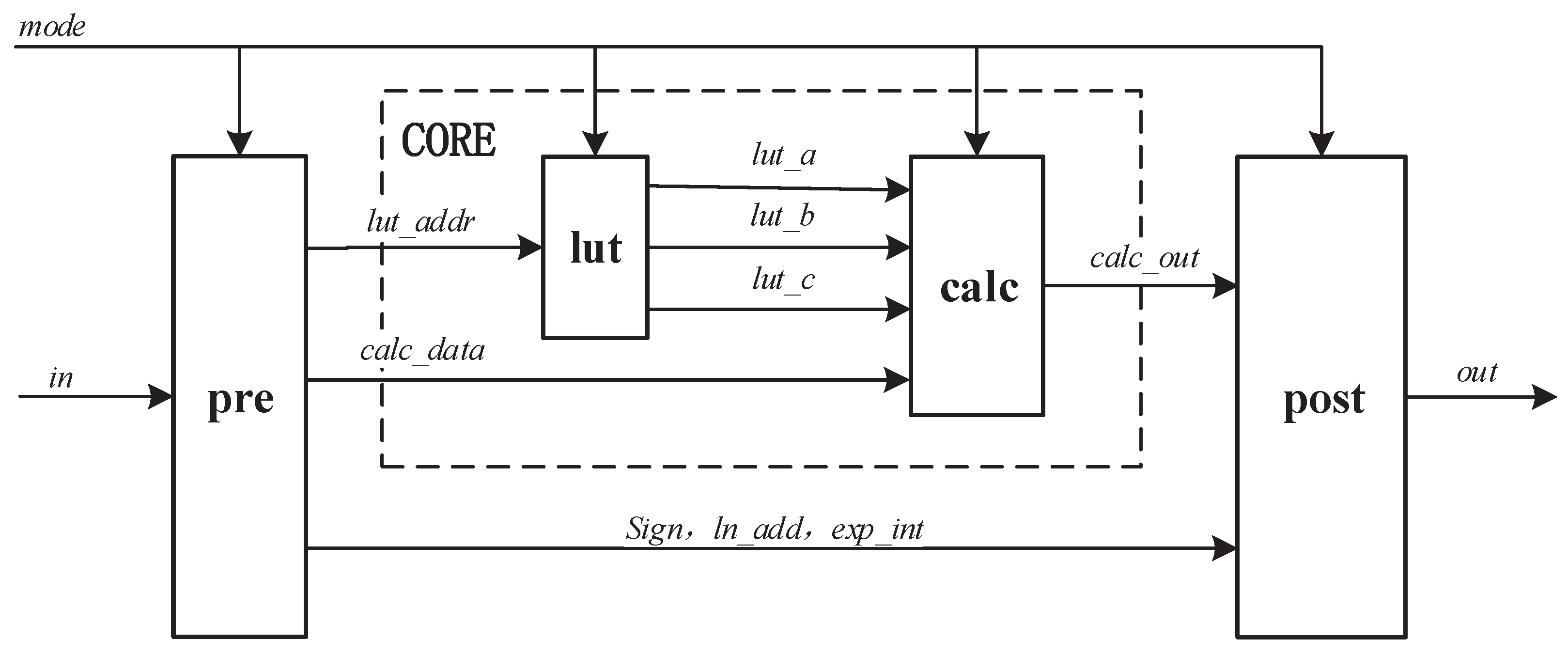
Reconfigurable Architecture: One Module, Five Functions
Li et al. [1] showed that all five functions (sin, cos, arctan, e^x, ln) can share a single fixed-point polynomial computation unit. The key observation is that after range reduction, every function is approximated by a polynomial of the same degree evaluated on a bounded domain. The only differences are the coefficient set and the pre/post-processing steps.
The reconfigurable module uses a mode-select signal to route data through function-specific preprocessing and postprocessing while sharing one polynomial evaluator. The LUT stores coefficients for all five functions, totaling 3.75 KB.
One complication is pipeline alignment. The preprocessing path length differs between functions – sin/cos/arctan have shorter preprocessing than e^x/ln – which would otherwise require stall logic. Retiming moves pipeline registers across combinational logic boundaries to equalize path lengths without changing logical behavior.
Results from Li et al. [1] on UMC 40 nm CMOS, validated against IEEE-754:
| Metric | Value |
|---|---|
| Max frequency | 220 MHz |
| Power (full load) | 0.923 mW |
| Area | 1.40×10^4 μm² |
| LUT size | 3.75 KB |
| Accuracy | ≤ 2 ulp |
| Area reduction vs 5 separate modules | 47.99% |
| Power reduction vs 5 separate modules | 38.91% |
Per-function breakdown:
| Function | Pipeline stages | Area (μm²) | Latency (ns) | Power (mW) |
|---|---|---|---|---|
| Sine | 3 | 6802.79 | 13.04 | 0.3132 |
| Cosine | 3 | 6802.79 | 13.04 | 0.3132 |
| Arctan | 3 | 6187.03 | 13.04 | 0.3725 |
| Exp | 4 | 7976.67 | 17.39 | 0.6075 |
| Log | 4 | 5968.74 | 17.39 | 0.2630 |
The shared polynomial core occupies only 28.18% of total chip area. The rest is preprocessing and postprocessing logic, most of which is already function-specific and cannot be shared further.
FPGA Head-to-Head: Three Implementations
Mohamed et al. [2] implemented all three approaches – LUT-based, polynomial, and CORDIC – on an AMD Artix-7 XC7A100T FPGA using Verilog. The application was a sine chaotic map and the Enhanced Modified Logistic Map (EMLM), which is deliberately error-sensitive: chaotic maps amplify small numerical differences over many iterations, making them a good discriminator for floating-point approximation quality.
FPGA resource comparison:
| Method | Format | Slices | Slice LUTs | Flip-Flops | DSP blocks |
|---|---|---|---|---|---|
| LUT-based | 32-bit | 1185 | 4280 | — | 0 |
| Polynomial | 32-bit | 54 | 205 | — | 28 |
| CORDIC | 32-bit | 396 | 1459 | — | 0 |
Performance and accuracy:
| Method | Input range | Max freq (MHz) | Throughput (Gbps) | Chaotic quality (K) |
|---|---|---|---|---|
| LUT-based | [0:0.001:π/2] | 800 | 0.263 | 0.0014 |
| Polynomial | [0, π/2] | 250.718 | 0.776 | 0.3982 |
| CORDIC | [-π, π] | 408.138 | 0.580 | 0.6968 |
The chaotic quality metric K is from the 0-1 test: K=1 indicates fully chaotic behavior, K≈0 indicates periodic or degraded dynamics. CORDIC achieves K=0.6968, closest to ideal. The LUT-based approach effectively collapses the chaotic dynamics (K=0.0014), likely due to quantization artifacts from the discrete lookup table. Polynomial sits in between.
Polynomial gives the highest throughput (0.776 Gbps) but consumes 28 DSP blocks. On an Artix-7, DSP blocks are a limited resource – 240 total on the XC7A100T. Spending 28 on a single function unit is expensive. CORDIC uses none.
LUT-based has the highest maximum frequency (800 MHz) because it is essentially a ROM read with no computation logic in the critical path, but it consumes the most slice LUTs and has the worst approximation accuracy for the chaotic map application.
Head-to-Head Summary
| Property | CORDIC | PR-CORDIC [3] | LUT+Poly [1] |
|---|---|---|---|
| Operations | Shift + Add | Shift + Add + Compare | Multiply + Add |
| Multipliers required | No | No | Yes |
| Iterations (single precision) | ≈ 24 | ≈ 14 | N/A (fixed pipeline) |
| Functions per module | 1 | 1 (arctan) | 5 (reconfigurable) |
| Frequency | Platform-dependent | Platform-dependent | 220 MHz (40 nm) |
| Power | Low | Low | 0.923 mW |
| Accuracy | ~1 bit/iter | Same | ≤ 2 ulp |
| Chaotic map quality | Best | — | Good |
| Throughput | Lower | Improved | 0.78 Gbps |
| Area for 5 functions | 5× module | 5× module | 47.99% less |
When to Use Which
The choice is not a question of correctness – both approaches can achieve single-precision accuracy. It is a question of resource profile.
Use CORDIC when multipliers are scarce. Many mid-range FPGAs have far more LUT fabric than DSP blocks. CORDIC uses only adders and shifts, which map entirely to LUTs. On a device where DSP blocks are already committed to a data processing pipeline, CORDIC is the only viable option for transcendental computation.
Use CORDIC when only one or two functions are needed. The area advantage of LUT+Polynomial comes from sharing a polynomial evaluator across five functions. If only sin and cos are needed, CORDIC computes both in the same pass. There is no shared-area benefit from LUT+Polynomial for one or two functions.
Use CORDIC in error-sensitive dynamic systems. The chaotic map results show that CORDIC produces more faithful numerical behavior than a discrete coefficient table when the computation feeds back on itself over many iterations. The error in CORDIC is smooth and distributed across iterations; LUT quantization introduces discontinuities at sub-interval boundaries.
Use LUT+Polynomial when multiple functions share a common module. The 47.99% area reduction over five separate accelerators is significant in silicon. If an application needs sin, cos, arctan, exp, and ln – which is common in DSP front-ends and ML inference pipelines – the reconfigurable polynomial architecture of Li et al. [1] delivers better area and power than five independent CORDIC units.
Use LUT+Polynomial when throughput is the primary constraint. A fully pipelined polynomial evaluator with Horner’s method has a short, fixed critical path: a chain of multiplier-adder stages. At 220 MHz on 40 nm CMOS with 3-4 pipeline stages, that is 660–880 million operations per second per function. CORDIC in pipelined mode achieves comparable throughput but at 24 pipeline stages and much more area.
Multipliers
available?
    │
    ├── Yes ──► Need > 2 functions?
    │               │
    │               ├── Yes ──► LUT + Polynomial (Li 2023 style)
    │               │
    │               └── No  ──► LUT + Polynomial
    │
    └── No  ──► Need > 2 functions?
                    │
                    ├── Yes ──► LUT + Polynomial (if LUT memory available)
                    │
                    └── No  ──► CORDIC (or PR-CORDIC)
Numerical Precision in Fixed-Point CORDIC
The precision of a fixed-point CORDIC implementation depends on three parameters: the internal datapath width (WIDTH), the iteration count (ITER), and the fractional precision of angle representation (FRAC). These interact non-independently.
From the parameterization sweep across a full synthesis characterization covering all six modes:
| Parameter | Minimum for < 1×10^-4 RMS | Notes |
|---|---|---|
| ITER | 16 | Beyond 16 yields no measurable improvement at 30-bit precision |
| WIDTH | 32 | WIDTH=40 with mismatched scaling produces catastrophic failure |
| FRAC | 28 | Required for sin/cos/magnitude below 10^-4 RMS |
The interaction between WIDTH and output scaling is a common failure mode. Output scaling mismatches (wrong OUT_SHIFT value) produce deterministic catastrophic failure – RMS error saturates near 0.7-1.2 – not gradual degradation. The failure looks identical whether the shift is off by one in either direction. This is because a wrong shift is a factor-of-two error in the output, which completely swamps the approximation error. The diagnostic signature is RMS error near 0.7-1.2 regardless of ITER or FRAC.
Accuracy at the production configuration (WIDTH=32, ITER=16, FRAC=30):
| Mode | Function | Max Error | RMS Error |
|---|---|---|---|
| Circular rotation | sin | 6.9×10^-5 | 3.9×10^-5 |
| Circular rotation | cos | 7.2×10^-5 | 3.9×10^-5 |
| Circular vectoring | magnitude | 5.6×10^-5 | 2.6×10^-5 |
| Linear rotation | multiply | 2.7×10^-5 | 9.2×10^-6 |
| Hyperbolic rotation | sinh | 1.1×10^-4 | 5.7×10^-5 |
| Hyperbolic rotation | cosh | 7.9×10^-5 | 4.3×10^-5 |
| Hyperbolic rotation | exp | 2.5×10^-4 | 1.1×10^-4 |
| Hyperbolic vectoring | ln | 1.5×10^-4 | 8.1×10^-5 |
The ill-conditioned cases deserve mention. tan(x) has unbounded error near ±π/2 because the denominator goes to zero and the fixed-point representation cannot represent the result. atan2 has large error near (0, 0) for the same reason – the angle of a zero-magnitude vector is undefined. These are not implementation bugs; they are fundamental singularities that any fixed-point implementation must guard against at the system level.
The hyperbolic mode requires the repeat schedule. Without it, the series diverges regardless of ITER or precision. The diagnostic for missing repeat schedule is outputs that appear to converge initially and then drift away from the correct value at larger input magnitudes.
Applications and Where CORDIC Shows Up in Real Systems
FFT twiddle factors. A radix-2 DIT FFT for N=8 requires N/2 = 4 complex twiddle factors W_N^k = e^{-j2πk/N}. These are fixed values that can be precomputed, but a CORDIC rotation mode computes them directly in hardware: for each k, set z_0 = -2πk/N and run rotation mode. N/2 parallel CORDIC instances can compute all twiddle factors in the same time as one, feeding the butterfly datapath with one result per clock. The benefit over a precomputed ROM is that the precision can be changed by adjusting WIDTH and ITER parameters without resizing a stored table.
Carrier recovery in QAM demodulation. A 16-QAM demodulator requires a Costas loop for carrier phase tracking. The phase error at each symbol is atan2(Q, I) – exactly the circular vectoring mode output. A second CORDIC instance in rotation mode drives the NCO (numerically controlled oscillator) for carrier synthesis. Both operations share the same core parameterization, which simplifies IP integration.
Digital PLL. A second-order DPLL for carrier recovery uses CORDIC rotation to synthesize the reference carrier. The phase detector uses a cross-product (Im{conj(nco) × ref}) rather than CORDIC vectoring, to avoid the ±180° false-lock ambiguity that arises when CORDIC preconditioning fails at large phase errors in a free-running loop.
Sigma-Delta ADC with digital downconversion. A bandpass oversampling ADC pipeline uses CORDIC in rotation mode as the NCO and mixer for shifting the IF output to baseband IQ. The angular input to the NCO is the phase increment; the complex output drives IQ routing. This is the same carrier recovery path as QAM demodulation, making the CORDIC IP drop-in compatible between the two.
GNSS coordinate transforms. Converting between ECEF (Earth-Centered, Earth-Fixed) and geodetic coordinates requires sin and cos of latitude and longitude at single-precision accuracy. CORDIC handles this with no floating-point hardware.
ML inference activations. Softmax requires e^x. GELU requires erf, which is closely related to sinh and can be approximated using hyperbolic CORDIC mode. As inference moves to specialized silicon and away from general-purpose GPU cores, transcendental function units become first-class design components rather than library calls.
Limitations of these works…
This post focuses on the algorithmic and architectural level. Several important directions are not covered here.
Faithfully rounded results. The IEEE-754 standard technically requires the four basic operations (add, subtract, multiply, divide) to be correctly rounded – the result must be the floating-point number nearest to the mathematical result. For transcendental functions, IEEE-754 only recommends but does not require correct rounding. Achieving correctly rounded transcendental results requires multi-precision intermediate computation and careful analysis of rounding errors, which is an active research area distinct from the approximation accuracy discussed here.
Posit arithmetic. The posit number system is an alternative to IEEE-754 that provides more precision near one and less near zero and infinity, motivated by the observation that most numerical computations operate near unit magnitude. CORDIC and polynomial approximation both have natural extensions to posit, but the precision analysis and range reduction steps differ.
bfloat16 and FP8. ML training uses 16-bit and 8-bit floating-point formats that trade precision for memory bandwidth. Transcendental function units for these formats have much lower precision requirements and can use shorter polynomial approximations or smaller CORDIC iteration counts, but the range reduction and exponent handling still apply.
Verification of numerical properties. This post covers formal verification of control and structural properties. Verifying that sin(x) is accurate to 2 ulp for all representable inputs is a different problem, typically addressed through exhaustive simulation or interval arithmetic, not bounded model checking.
Summary
Two algorithmic families dominate hardware transcendental function computation. CORDIC uses only shifts and additions, requires no multipliers, and produces two function outputs for the cost of computing one. Its precision scales linearly with iteration count: approximately one bit per iteration, requiring 24 iterations for single-precision. It is the right choice for resource-constrained FPGAs, DSP systems that only need a few functions, and applications where smooth numerical behavior across the full input range matters more than peak throughput.
LUT+Polynomial requires multipliers but delivers higher throughput with a fixed, short pipeline depth. The key architectural insight from Li et al. [1] is that all five transcendental functions share the same polynomial evaluation core – only the coefficients differ. Sharing this core across five functions yields 47.99% area reduction and 38.91% power reduction compared to five separate accelerators. This is the right approach when multipliers are available and multiple functions are needed simultaneously.
PR-CORDIC reduces the iteration count from 24 to 14 for single precision by adding pre-rotation logic, closing approximately half the latency gap between CORDIC and polynomial at modest area cost. It currently covers arctangent; extension to the full trigonometric set remains an open implementation task.
The FPGA comparison of Mohamed et al. [2] makes the practical tradeoffs concrete: polynomial achieves 0.776 Gbps throughput at the cost of 28 DSP blocks; CORDIC achieves 0.580 Gbps with zero DSPs and significantly better behavior in error-sensitive applications; pure LUT achieves 800 MHz but degrades approximation quality for dynamic systems.
Neither approach is universally superior. The right choice is determined by available resources on the target platform and the application’s sensitivity to area, power, throughput, and numerical precision.
References
[1] P. Li, H. Jin, W. Xi, C. Xu, H. Yao, and K. Huang, “A reconfigurable hardware architecture for miscellaneous floating-point transcendental functions,” Electronics, vol. 12, no. 1, Art. no. 233, 2023. DOI: 10.3390/electronics12010233
[2] S. M. Mohamed, M. H. Yacoub, W. S. Sayed, L. A. Said, and A. G. Radwan, “Efficient hardware implementations of trigonometric functions and their application to sine-based modified logistic map,” Digital Signal Processing, vol. 159, Art. no. 104993, 2025. DOI: 10.1016/j.dsp.2025.104993
[3] K. Li, H. Fang, Z. Ma, F. Yu, B. Zhang, and Q. Xing, “A low-latency CORDIC algorithm based on pre-rotation and its application on computation of arctangent function,” Electronics, vol. 13, no. 12, Art. no. 2338, 2024. DOI: 10.3390/electronics13122338
[4] M. Song et al., “A design of transcendental function accelerator,” in Proc. SPIE, Third International Conference on Artificial Intelligence and Computer Engineering (ICAICE 2022), vol. 12610, Art. no. 1261002, 2023.
[5] J. Wei and H. Kobayashi, “A review of floating-point arithmetic algorithms using Taylor series expansion and mantissa region division techniques,” Preprints, 2026, Art. no. 202601.0284.
[6] J. Volder, “The CORDIC trigonometric computing technique,” IRE Transactions on Electronic Computers, vol. EC-8, no. 3, pp. 330–334, 1959.