Floating Point vs Fixed Point: A Hardware-Centric Perspective
In software, numeric representation is abstract. In hardware, numeric representation is architecture.
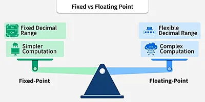
Choosing between floating point and fixed point is not about syntax — it is about:
- Silicon area
- Power consumption
- Latency
- Determinism
- Quantization behavior
- Verification complexity
This article examines both representations from a digital hardware perspective.
What Is Floating Point?
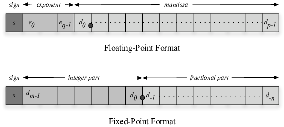
Floating point represents numbers in scientific notation:
\[ x = (-1)^s \times 1.m \times 2^e \]
Where:
- \( s \) = sign bit
- \( m \) = mantissa
- \( e \) = exponent
The dominant standard is IEEE 754.
IEEE 754 Single Precision (32-bit)
| Field | Bits |
|---|---|
| Sign | 1 |
| Exponent | 8 |
| Mantissa | 23 |
Double precision uses 64 bits.
Floating point provides:
- Large dynamic range
- Automatic scaling
- Relative precision
Where Floating Point Fails
Consider:
\[ x = 1.000001 \]
Now scale:
\[ y = x - 1 \]
In floating point, when numbers are very close, subtracting nearly equal values causes catastrophic cancellation. Precision collapses.
Similarly:
\[ 10^8 + 1 - 10^8 \]
May not return 1 exactly due to mantissa limits.
Floating point preserves dynamic range, not absolute precision.
Hardware Cost of Floating Point
Floating-point addition requires:
- Exponent alignment
- Mantissa shifting
- Leading-zero detection
- Normalization
- Rounding logic
Floating-point multiplication requires:
- Mantissa multiplication
- Exponent addition
- Normalization
- Rounding
In FPGA or ASIC:
- Large combinational logic
- Wide shifters
- Barrel shifters
- DSP + control logic
Latency is multi-cycle. Area is significant. Power increases.
Floating-point units (FPUs) are complex subsystems.
Fixed Point Representation
Fixed point represents numbers as integers scaled by a constant factor.
\[ x_{real} = \frac{x_{integer}}{2^F} \]
Where:
- \( F \) = number of fractional bits
There is no exponent. Scaling is implicit.
Q Notation (Critical for Hardware)
Fixed-point numbers are described using Q format:
\[ Qm.n \]
Where:
- \( m \) = integer bits (excluding sign)
- \( n \) = fractional bits
- Total bits = \( 1 + m + n )
Example:
Q1.15 (16-bit signed)
- 1 integer bit
- 15 fractional bits
- Range: \[ -2 \le x < 2 \]
Resolution: \[ \Delta = 2^{-15} \approx 3.05 \times 10^{-5} \]
Example Formats
| Format | Range | Resolution |
|---|---|---|
| Q1.7 | -2 to <2 | (2^{-7} = 0.0078) |
| Q3.12 | -8 to <8 | (2^{-12} \approx 0.000244) |
| Q7.8 | -128 to <128 | (2^{-8} = 0.0039) |
Tradeoff:
More fractional bits → better precision More integer bits → larger dynamic range
But total width increases hardware cost.
Revisit the Previous Example in Fixed Point
Take:
\[ x = 1.000001 \]
Using Q1.15:
Quantized value:
\[ 1.000001 \approx 1.000000 \quad (\text{rounded}) \]
Error ≈ \( 3 \times 10^{-5} )
Using Q1.7:
\[ 1.000001 \approx 1.0000 \]
Error ≈ 0.0078
Thus:
| Format | Error |
|---|---|
| Float (32-bit) | ~1e-7 |
| Q1.15 | ~3e-5 |
| Q1.7 | ~7.8e-3 |
Fixed point loses precision deterministically.
But error is bounded and predictable.
Small C++ Example
#include <iostream>
#include <cmath>
#include <cstdint>

int main() {
    float a = 1.000001f;
    float b = a - 1.0f;

    // Fixed Q1.7
    int16_t q7 = round(a * 128);
    float q7_real = q7 / 128.0f;
    float q7_err = fabs(a - q7_real);

    // Fixed Q1.15
    int32_t q15 = round(a * 32768);
    float q15_real = q15 / 32768.0f;
    float q15_err = fabs(a - q15_real);

    std::cout << "Float result: " << b << std::endl;
    std::cout << "Q1.7 error: " << q7_err << std::endl;
    std::cout << "Q1.15 error: " << q15_err << std::endl;
}
Sample Observed Output
Float result: 0.0000010
Q1.7 error: 0.0078125
Q1.15 error: 0.0000305
Interpretation:
- Floating point maintains relative precision.
- Q1.15 is acceptable for DSP-level precision.
- Q1.7 is coarse but hardware-efficient.
Hardware Tradeoffs (Critical Section)
Area
| Operation | Floating | Fixed |
|---|---|---|
| Add | Large | Small |
| Multiply | Very Large | Moderate (DSP) |
| Division | Very Large | Rarely used |
Floating point requires:
- Wide datapaths
- Exponent logic
- Normalization hardware
Fixed point:
- Simple adders
- Direct DSP mapping
- No exponent handling
Power
Floating point:
- Higher switching activity
- Larger combinational blocks
- More routing
Fixed point:
- Lower power
- Narrower buses
- Predictable switching
Latency
Floating:
- Multi-stage pipelines
- 3–8 cycles typical
Fixed:
- 1–2 cycles for add/multiply
Determinism
Floating:
- Rounding modes
- Denormal handling
- Edge-case complexity
Fixed:
- Deterministic overflow
- Predictable saturation
Overflow and Saturation
In fixed point:
If result exceeds representable range:
- Wraparound (two’s complement overflow)
- Saturation logic (clamp to max/min)
Hardware designers prefer saturation in DSP systems.
Floating point handles overflow via:
- Infinity
- NaN
Which complicates verification.
Non-Uniform Quantization
Floating point is effectively non-uniform quantization.
Resolution scales with magnitude:
\[ \Delta x \propto x \]
Large numbers:
- Coarser absolute precision
Small numbers:
- Finer absolute precision
Fixed point is uniform quantization:
\[ \Delta x = constant \]
Why Non-Uniform Quantization Is Powerful
In floating point:
- Relative error remains approximately constant
- Dynamic range is enormous
This is ideal for:
- Scientific computing
- Large dynamic simulations
Why Uniform Quantization Is Powerful
In fixed point:
- Noise floor predictable
- Hardware simple
- Excellent for bounded signals
Ideal for:
- DSP pipelines
- CNN accelerators
- FIR filters
- Motor control
Where Each Dominates
| Application | Preferred Format |
|---|---|
| Scientific simulation | Floating |
| Graphics rendering | Floating |
| Embedded DSP | Fixed |
| Neural network inference | Fixed (INT8/Q formats) |
| Control systems | Fixed |
| Training deep networks | Floating (FP32/FP16/BF16) |
Final Hardware Perspective
Floating point optimizes dynamic range and relative precision. Fixed point optimizes area, power, and latency.
In hardware design:
- Floating point costs silicon.
- Fixed point costs engineering effort (scaling decisions).
The decision is architectural.
If the signal range is bounded and known:
Fixed point is almost always superior.
If the dynamic range is unpredictable:
Floating point provides safety at silicon cost.
Understanding this distinction is essential for DSP engineers, ASIC designers, and ML hardware architects.