
Floating Point vs Fixed Point: A Hardware-Centric Perspective
In software, numeric representation is an abstraction you rarely have to think about. The compiler handles it, the hardware handles it, and the behavior is consistent across runs because the floating-point unit is already there. In hardware design, numeric representation is an architectural decision with direct consequences for silicon area, power consumption, pipeline depth, and verification complexity. Choosing between floating-point and fixed-point arithmetic is not a preference. It determines what your datapath looks like.
This post covers both representations from a hardware perspective: what they actually encode, what hardware is required to operate on them, where each one breaks down numerically, and which application domains favor each approach and why.
What Floating Point Actually Encodes
A floating-point number represents a value in scientific notation base 2:
\[ x = (-1)^s \times 1.m \times 2^{e - \text{bias}} \]
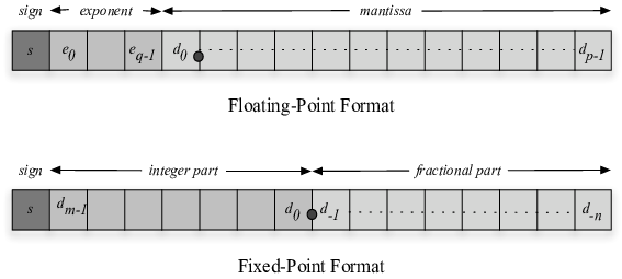
where s is the sign bit, m is the mantissa (the fractional part of the significand), and e is the stored biased exponent. The leading 1 before the binary point is implicit and not stored, which is why a 23-bit mantissa field gives 24 bits of significand precision.
IEEE 754 single precision uses 32 bits:
| Field | Width | Notes |
|---|---|---|
| Sign | 1 bit | 0 = positive, 1 = negative |
| Exponent | 8 bit | Biased by 127; range -126 to +127 |
| Mantissa | 23 bit | Implicit leading 1 |
This encodes values from approximately 1.2x10^-38 to 3.4x10^38, with roughly 7 decimal digits of relative precision throughout that range. IEEE 754 double precision extends the exponent to 11 bits and the mantissa to 52 bits, giving roughly 15 digits of relative precision and a range up to about 1.8x10^308.
The key property of this representation is that precision scales with magnitude. A value near 1.0 is represented with finer granularity than a value near 10^6, because both use the same 24-bit significand width but the exponent scales the step size between adjacent representable values. Two adjacent representable single-precision floats near 1.0 are about 1.2x10^-7 apart. Two adjacent representable floats near 10^6 are about 0.125 apart. This scaling is the source of floating-point’s dynamic range, and it is also the source of its most common failure mode.
Where Floating Point Fails Numerically
Floating-point arithmetic does not fail randomly. It fails in predictable ways that follow from the finite mantissa width.
Catastrophic cancellation is the most operationally dangerous case. When two nearly equal values are subtracted, the result has far fewer significant bits than either operand.
Consider computing x - 1 where x = 1.000001. In single precision, the value 1.000001 is representable with about 7 significant digits. After subtracting 1.0, the result should be 0.000001, which requires 7 significant digits to represent correctly but the subtraction has eliminated the leading ones that carried most of the precision. The result is 1.000001 - 1.000000 = 0.000001, but the floating-point subtraction leaves only about 1 significant digit because the significands aligned and then the common prefix cancelled. Any computation that subsequently uses this result as a divisor or an input to a function amplifies the error.
This is not a precision failure in the sense that the individual numbers were not represented accurately. The subtraction itself is performed correctly by the FPU. The precision loss is a consequence of the representation: the bits that encoded the difference between 1.000001 and 1.0 were in the least significant positions of the mantissa, and those are the bits that survive after the leading digits cancel.
Absorption happens when a small value is added to a much larger one and the small value is completely lost:
\[ 10^8 + 1 - 10^8 \]
In exact arithmetic this returns 1. In single-precision floating point, the addition 10^8 + 1 is evaluated first. The value 10^8 in single precision has its significant bits representing values of 1.0 and above in units of 8 (the spacing between adjacent floats near 10^8 is about 8), so the integer 1 is below the representable resolution at that magnitude. It rounds to zero. The result is 10^8 + 0 - 10^8 = 0, not 1.
Both of these failures are deterministic. For a given input, a given FPU produces the same wrong answer every time. But they are also non-obvious: the same sequence of operations applied to slightly different inputs may produce a completely correct result. This makes floating-point bugs difficult to reproduce and localize in hardware systems where the input stream is not controlled.
Hardware Cost of Floating-Point Operations
The cost of floating-point arithmetic in hardware is not proportional to the bit width in the way that integer arithmetic is. The operations require structural hardware beyond the arithmetic units themselves.
Floating-point addition requires five distinct phases: exponent comparison to determine the alignment shift, mantissa alignment by right-shifting the smaller operand’s significand by the exponent difference, the actual mantissa addition, leading-zero detection to determine how far the result must shift left to restore the implicit leading 1, and normalization by shifting left and decrementing the exponent. Each of these phases takes multiple gate delays, and the leading-zero detection and normalization steps require a priority encoder and a barrel shifter, both of which are wide combinational structures.
Floating-point multiplication is simpler structurally: the mantissas are multiplied (integer multiplication of two (1+23)-bit values giving a 48-bit product), the exponents are added and the bias is subtracted, and the result is normalized. The multiplication itself is the expensive part. A 24x24 multiplier requires either a large array multiplier or a sequence of partial product accumulation steps using DSP blocks.
Floating-point division is significantly more expensive than multiplication. Software FPUs typically use Newton-Raphson iteration (which still requires multiplications) or an SRT digit-recurrence algorithm. Hardware divide units are often not fully pipelined and have variable latency.
On an FPGA, a single-precision floating-point adder using Xilinx floating-point IP typically consumes 2-3 DSP blocks, several hundred LUTs, and has a pipeline depth of 5-7 cycles at a clock frequency around 300-400 MHz on a UltraScale device. A floating-point multiplier is slightly more expensive in DSP blocks. These numbers are from synthesis, not theoretical estimates, and they vary with device family and optimization settings. The point is that a single FP adder occupies a meaningful fraction of a mid-range FPGA device’s DSP budget, and a datapath with many floating-point operations consumes DSP blocks that are no longer available for other uses.
On an ASIC in a 28nm process, a single-precision FPU (add, subtract, multiply, fused multiply-add) occupies approximately 10,000-30,000 gates depending on pipeline depth and feature set. A divide unit roughly doubles this. Compared to a 32-bit integer ALU at around 2,000-5,000 gates, floating-point is expensive silicon.
Fixed-Point Representation
Fixed-point represents a value as a scaled integer:
\[ x_{\text{real}} = x_{\text{integer}} \times 2^{-F} \]
where F is the number of fractional bits. There is no exponent field. There is no normalization. The binary point is fixed at a position determined by the designer at design time, and it never moves during computation. The hardware treats the value as an ordinary integer; the interpretation of where the binary point sits is a software convention that the hardware is not aware of.
Q Notation
Fixed-point formats are described using Q notation:
\[ Qm.n \]
where m is the number of integer bits (not counting the sign bit) and n is the number of fractional bits. The total bit width is 1 + m + n for a signed format.
Q1.15 is a 17-bit signed format: 1 sign bit, 1 integer bit, 15 fractional bits. Range is -2 to just under +2, with resolution 2^-15 = 3.05x10^-5. This format is standard in 16-bit DSP arithmetic where the signed 16-bit value is interpreted as Q1.15 by convention.
Q3.12 is a 16-bit signed format: 1 sign bit, 3 integer bits, 12 fractional bits. Range is -8 to just under +8, resolution 2^-12 = 2.44x10^-4. This covers a wider range than Q1.15 at the cost of reduced fractional precision.
| Format | Total width | Range | Resolution |
|---|---|---|---|
| Q1.7 | 9-bit signed | -2 to <2 | 2^-7 = 0.0078 |
| Q1.15 | 17-bit signed | -2 to <2 | 2^-15 = 3.05x10^-5 |
| Q3.12 | 16-bit signed | -8 to <8 | 2^-12 = 2.44x10^-4 |
| Q7.8 | 16-bit signed | -128 to <128 | 2^-8 = 0.0039 |
| Q15.0 | 16-bit signed | -32768 to 32767 | 1 (integer) |
The tradeoff within a fixed total width is always between dynamic range (integer bits) and precision (fractional bits). The designer commits to this tradeoff at design time based on the signal range of the application. If the signal occasionally exceeds the representable range, the result saturates or wraps, neither of which is quiet like a floating-point infinity.
Quantization Error
Fixed-point quantization error is deterministic and bounded. For a Q format with n fractional bits, the maximum quantization error for any representable input is 2^-(n+1) with rounding or 2^-n with truncation. This error is uniform across the entire representable range, which is both a limitation and a strength.
Returning to the previous example: representing x = 1.000001 in Q1.15:
The exact value is 1.000001. The closest Q1.15 value is round(1.000001 x 32768) / 32768 = 32768 / 32768 = 1.000000. Quantization error is approximately 3x10^-5, which is about 3 least-significant bit widths at Q1.15 resolution.
In single-precision floating point, the same value is represented with error approximately 1.2x10^-7. Floating point wins on precision for this specific value by about two orders of magnitude, using the same number of bits (32 for float vs 17 for Q1.15). But the comparison is not fair on equal bit widths. A 32-bit fixed-point format Q1.30 represents this value with error 2^-31 = 9.3x10^-10, which is better than single-precision float. The question is always what the signal range requires.
#include <iostream>
#include <cmath>
#include <cstdint>

int main() {
    float a = 1.000001f;

    // Floating point subtraction -- catastrophic cancellation
    float b = a - 1.0f;

    // Fixed Q1.7: 1 integer bit, 7 fractional bits
    int16_t q7 = (int16_t)round(a * 128.0f);
    float q7_real = q7 / 128.0f;
    float q7_err = fabsf(a - q7_real);

    // Fixed Q1.15: 1 integer bit, 15 fractional bits
    int32_t q15 = (int32_t)round(a * 32768.0f);
    float q15_real = q15 / 32768.0f;
    float q15_err = fabsf(a - q15_real);

    std::cout << "Float (a - 1.0f):   " << b      << std::endl;
    std::cout << "Q1.7 quant error:   " << q7_err  << std::endl;
    std::cout << "Q1.15 quant error:  " << q15_err << std::endl;
}
Float (a - 1.0f):   9.99991e-07
Q1.7 quant error:   0.0078125
Q1.15 quant error:  3.05176e-05
The floating-point result of a - 1.0f is approximately correct at about 1x10^-6. The Q1.15 quantization error is 3x10^-5. Both represent 1.000001 with error; floating-point tracks the value more accurately per bit in this particular case because the mantissa concentrates precision near 1.0. Q1.7 has an error of nearly 8x10^-3, which is acceptable for rough DSP work but not for precision control systems.
The important distinction is that both Q1.7 and Q1.15 errors are known at design time. Before the hardware runs a single cycle of simulation, the maximum quantization error is computable analytically. Floating-point error, especially after operations that cause cancellation or absorption, is not bounded in the same way without careful floating-point error analysis of the specific computation.
Hardware Cost: The Direct Comparison
Addition. A fixed-point adder for two N-bit operands is an N-bit carry-propagate adder. For N = 16, this is 16 full adder stages. The critical path is approximately log2(16) gate delays with a carry lookahead structure. A floating-point adder for 32-bit IEEE 754 requires exponent subtraction, a barrel shifter with up to 23-bit shift distance, the significand addition, a leading-zero encoder, another barrel shifter for normalization, and rounding logic. The FP adder’s gate count is roughly 15-25x that of a 32-bit integer adder.
Multiplication. A fixed-point multiplier for two N-bit operands produces a 2N-bit product and requires an N x N partial product tree. For N = 16, this maps directly to one DSP block on most FPGAs. A floating-point 32-bit multiplier requires a 24 x 24 significand multiplication plus exponent addition and normalization. On an FPGA, this typically requires 3 DSP blocks plus additional LUTs for exponent handling and normalization.
Division. Fixed-point division is rarely implemented in hardware for DSP applications. Where a reciprocal or division is needed, it is pre-computed as a fixed-point constant and replaced with a multiply-shift sequence. Floating-point division is implementable in hardware but expensive: a typical implementation uses Newton-Raphson iteration over 2-3 multiplications, or a digit-recurrence algorithm requiring many clock cycles. Neither is cheap.
| Operation | Fixed-point cost | Floating-point cost |
|---|---|---|
| Add (16/32 bit) | 1 adder, 1-2 cycle latency | ~20x gate count, 5-7 cycle latency |
| Multiply (16-bit fixed) | 1 DSP block | 3+ DSP blocks |
| Divide | Rarely used (precomputed reciprocal) | Expensive; 10-20+ cycles |
Power. Floating-point datapaths consume more power than fixed-point at the same clock frequency for three reasons. The wider datapaths switch more bits per operation. The normalization and rounding logic is active on every result. The barrel shifters in the add and result paths are wide combinational networks with significant switching activity. In an application-specific accelerator for a power-constrained application, this difference is significant. Neural network inference chips use fixed-point arithmetic (INT8 or INT4) explicitly because the power reduction from eliminating floating-point hardware across thousands of parallel multipliers is substantial.
Overflow and Saturation
Fixed-point arithmetic overflows when the result of an operation exceeds the representable range. Two’s complement wraparound is the default behavior of integer hardware: if a 16-bit result would be 32800 (beyond the Q1.15 range of approximately 32767), the hardware produces -32736 instead. This is arithmetically wrong and produces a signal polarity inversion, which can destabilize control loops or corrupt audio pipelines in ways that are difficult to diagnose.
The standard solution in DSP hardware is saturation: if the result would overflow, clamp it to the maximum representable value instead of wrapping.
// Saturating adder for 16-bit signed fixed-point
wire signed [16:0] sum = {a[15], a} + {b[15], b};  // 17-bit to catch overflow
wire overflow_pos = ~sum[16] & sum[15];  // Result would be too positive
wire overflow_neg =  sum[16] & ~sum[15]; // Result would be too negative

assign result = overflow_pos ? 16'sh7FFF :
                overflow_neg ? 16'sh8000 :
                sum[15:0];
The saturation logic adds comparators and muxes after each arithmetic result. It is standard practice in DSP pipelines for audio processing, filter banks, and control system implementations where signal clipping at the boundary is preferable to polarity reversal from wraparound.
Floating-point handles overflow by producing infinity or NaN. Infinity propagates through subsequent operations in defined ways: infinity plus any finite value is infinity, and so on. NaN propagates through all operations without producing a hardware exception by default in most FPU configurations. This makes floating-point overflow quieter than fixed-point overflow, but it also means that a NaN injected early in a computation pipeline can propagate silently through many subsequent operations before producing an obviously wrong output. Detecting NaN propagation in a deep pipeline requires explicit NaN checks at intermediate points, which complicates the verification effort.
Uniform vs Non-Uniform Quantization
Fixed-point is uniform quantization. The spacing between adjacent representable values is constant everywhere in the representable range:
\[ \Delta x = 2^{-F} \quad \text{(constant for all } x \text{)} \]
A Q1.15 format has exactly the same resolution at x = 0.0001 as at x = 1.9999. The quantization noise power is uniform across the signal range.
Floating-point is non-uniform quantization. The spacing between adjacent representable values scales with the magnitude of the value:
\[ \Delta x \approx |x| \times 2^{-(p-1)} \]
where p is the significand precision in bits (24 for single precision). Near x = 1.0, the spacing is about 1.2x10^-7. Near x = 10^6, the spacing is about 0.125. The relative precision is approximately constant; the absolute precision varies by six orders of magnitude across the single-precision range.
This non-uniform distribution is the right choice when the signal has unpredictable dynamic range and relative accuracy matters more than absolute accuracy. Scientific simulations, rendering computations, and training deep networks all fall in this category because the values being computed span many orders of magnitude and the computation requires that relative errors stay small.
Fixed-point’s uniform quantization is the right choice when the signal is bounded and the noise floor must be predictable. An FIR filter coefficient set is designed with the assumption that the filter input signal amplitude is within a defined range. The filter’s frequency response deviation due to coefficient quantization is predictable from the Q format and the filter order. A floating-point FIR filter would have lower coefficient quantization error, but the added hardware cost provides no benefit because the signal is already bounded by design.
Where Each Format Dominates
The choice between floating-point and fixed-point is driven by the application, the hardware budget, and the signal characteristics. There is no universally superior choice.
| Application | Standard format | Reason |
|---|---|---|
| DSP filter banks | Fixed, Q1.15 or Q3.12 | Bounded signals, uniform noise floor |
| Neural network inference | Fixed, INT8 or INT4 | Power and area, accuracy sufficient after quantization-aware training |
| Neural network training | Float, FP32 or BF16 | Wide dynamic range in gradients, precision needed for convergence |
| Motor control | Fixed, Q15 or Q31 | Real-time, bounded signals, deterministic latency |
| GNSS receiver baseband | Fixed, Q1.15 | Narrow dynamic range after AGC, DSP blocks map directly |
| Scientific simulation | Float, FP64 | Unbounded dynamic range, relative precision required |
| Graphics rendering | Float, FP32 or FP16 | Coordinate values span many orders of magnitude |
| Audio codec | Fixed, Q1.23 or Q1.31 | High dynamic range needed, but signal is bounded by full-scale |
The application categories that default to fixed-point share a common characteristic: the signal has a known, bounded amplitude range at design time. When the range is bounded, the designer can select a Q format that covers the range with sufficient headroom and uses the remaining bits for fractional precision. The hardware then needs no exponent handling, no normalization, and no rounding unit beyond truncation or saturation.
The categories that require floating-point share a different characteristic: the values span a dynamic range that cannot be bounded at design time, or the relative precision requirements are strict enough that the non-uniform quantization of floating-point is necessary to maintain accuracy throughout the computation.
Mixed Formats in Real Systems
Many practical hardware systems use both formats in different parts of the pipeline. A DSP beamforming processor might perform all channel processing in Q1.15 fixed-point but use floating-point for the final spatial FFT where the dynamic range of the beamformed output is difficult to predict without knowing the channel geometry. An ML inference chip uses INT8 fixed-point for convolution layers (the bulk of the computation) but may use FP32 or FP16 for the softmax normalization at the output layer, where the exponential values span a wide range.
This mixing requires explicit format conversion hardware at the boundary between fixed-point and floating-point sections of the datapath. Integer-to-float conversion and float-to-integer conversion both take multiple clock cycles and are not free in area. The placement of format conversion boundaries is an architectural decision that affects both the data path and the pipeline control logic.
Summary
Floating-point encodes relative precision: the step size between adjacent values scales with the magnitude of the value, giving approximately constant relative error across a wide dynamic range. Fixed-point encodes absolute precision: the step size is constant everywhere, giving bounded, predictable quantization error for signals whose amplitude range is known.
The hardware cost of floating-point is substantially higher for every operation. A floating-point adder is 15-25x more expensive in gate count than a fixed-point adder at the same effective precision. A floating-point multiplier requires 3x more DSP blocks than a fixed-point multiplier operating on the same-width operands. Power consumption is correspondingly higher.
Fixed-point costs engineering time rather than silicon. The designer must analyze the signal range, select the Q format, verify that overflow does not occur in any reachable state, implement saturation where necessary, and re-analyze whenever the signal processing chain changes. This is analytical work that does not show up in gate count but is real design effort.
For hardware with bounded input signals, fixed-point is the right choice in nearly every case. The precision difference is recoverable by adding more fractional bits, the hardware savings are substantial, and the quantization behavior is predictable. For hardware that must handle unbounded dynamic range or requires the precision properties of floating-point at specific points in the computation, the area and power cost of floating-point hardware is the price of correctness.