Machine learning in physical design (PD) is not about replacing routing or timing engines. It is about predicting expensive post-route outcomes earlier in the flow.

Inside PD, the questions are:

• Will this placement cause routing congestion?
• Where will DRC violations cluster?
• Which regions will suffer IR drop?
• What will be the net delay before detailed routing?

All of these are spatial or graph-structured problems. That is why most modern approaches convert PD data into:

• Image-like tensors (grid-based Gcells)
• Graph representations (nets and pins)

This post explains:

• What to train for each PD task
• Why each feature exists
• How features are constructed
• What model architecture to use
• How to wire the full training code

No metrics. No benchmarking. Only feature reasoning and implementation.

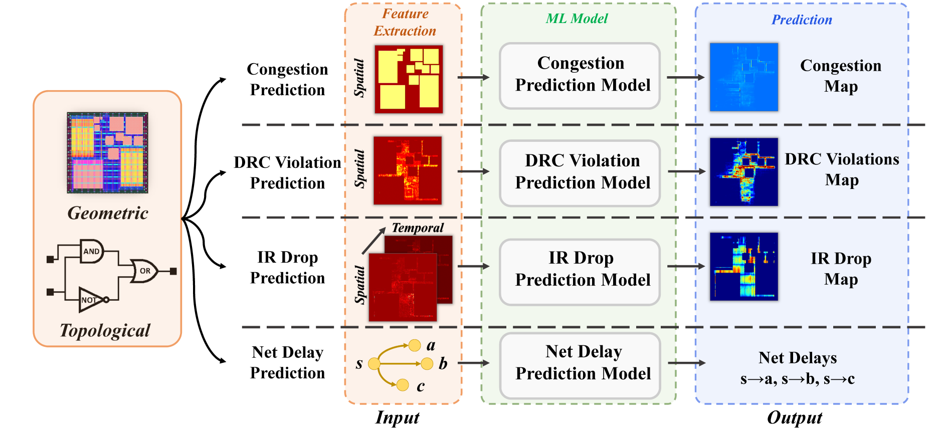
Congestion Prediction in PD

Congestion is routing demand exceeding routing resources during global routing.

In PD terms:

\[ Congestion = \frac{Routing\ Demand}{Routing\ Capacity} \]

If overflow > 0 → hotspot.

We want to predict congestion at placement stage before routing.

This becomes an image-to-image regression problem.

Input: feature maps over layout grid Output: horizontal + vertical overflow maps

Features Used for Congestion

Three features are sufficient and meaningful:

macro_region

This is a binary or density map indicating macro block locations.

Why it matters:

• Macros block routing tracks.
• They create routing detours.
• Pin access around macros is restricted.
• High macro density increases congestion probability.

Without macro_region, the model cannot learn structural routing barriers.

RUDY (Rectangular Uniform Wire Density)

RUDY estimates routing demand based on net bounding boxes.

Concept:

For each net:

\[ RUDY = \frac{Net\ Degree}{Bounding\ Box\ Area} \]

High RUDY means many nets compressed into small region.

Why it matters:

• Approximates routing demand before routing.
• Encodes net topology implicitly.
• Strong indicator of congestion clusters.

RUDY_pin

Similar to RUDY but weighted by pin density.

Why it matters:

• Regions with high pin concentration require more vias and routing tracks.
• Pin access complexity drives congestion.
• Captures cell-level granularity.

Model Architecture (FCN Encoder–Decoder)

We treat layout as an image.

Encoder extracts spatial patterns. Decoder reconstructs congestion map.

Full model:

import torch
import torch.nn as nn

class conv(nn.Module):
    def __init__(self, dim_in, dim_out):
        super().__init__()
        self.main = nn.Sequential(
            nn.Conv2d(dim_in, dim_out, 3, 1, 1),
            nn.InstanceNorm2d(dim_out, affine=True),
            nn.LeakyReLU(0.2, inplace=True),
            nn.Conv2d(dim_out, dim_out, 3, 1, 1),
            nn.InstanceNorm2d(dim_out, affine=True),
            nn.LeakyReLU(0.2, inplace=True),
        )
    def forward(self, x):
        return self.main(x)

class Encoder(nn.Module):
    def __init__(self, in_dim):
        super().__init__()
        self.c1 = conv(in_dim, 32)
        self.pool1 = nn.MaxPool2d(2)
        self.c2 = conv(32, 64)
        self.pool2 = nn.MaxPool2d(2)
        self.c3 = nn.Conv2d(64, 32, 3, 1, 1)

    def forward(self, x):
        h1 = self.c1(x)
        h2 = self.pool1(h1)
        h3 = self.c2(h2)
        h4 = self.pool2(h3)
        h5 = torch.tanh(self.c3(h4))
        return h5, h2

class Decoder(nn.Module):
    def __init__(self):
        super().__init__()
        self.up1 = nn.ConvTranspose2d(32, 16, 4, 2, 1)
        self.c1 = conv(16, 16)
        self.up2 = nn.ConvTranspose2d(16+64, 4, 4, 2, 1)
        self.out = nn.Conv2d(4, 2, 3, 1, 1)

    def forward(self, x):
        feat, skip = x
        x = self.up1(feat)
        x = self.c1(x)
        x = self.up2(torch.cat([x, skip], dim=1))
        return torch.sigmoid(self.out(x))

class GPDL(nn.Module):
    def __init__(self):
        super().__init__()
        self.encoder = Encoder(3)
        self.decoder = Decoder()

    def forward(self, x):
        return self.decoder(self.encoder(x))

Training:

model = GPDL().cuda()
optimizer = torch.optim.Adam(model.parameters(), lr=1e-4)

for feature, label in loader:
    feature = feature.cuda()
    label = label.cuda()
    pred = model(feature)
    loss = nn.MSELoss()(pred, label)
    optimizer.zero_grad()
    loss.backward()
    optimizer.step()

Label: congestion_GR_horizontal_overflow congestion_GR_vertical_overflow

DRC Violation Prediction in PD

DRC violations appear after detailed routing.

Congestion is coarse. DRC violations are technology-aware.

Advanced nodes introduce:

• Spacing violations
• Via enclosure violations
• Min-width violations

Predicting DRC directly avoids routing iteration loops.

Features Used for DRC

Nine features:

macro_region

Same reasoning as congestion.

cell_density

Density of standard cells per tile.

Why it matters:

• High density → narrow routing channels.
• Increased via stacking.
• High probability of spacing violations.

RUDY_long and RUDY_short

Split nets by span length.

• Long nets → global routing stress.
• Short nets → local routing congestion.

Separating them allows model to learn different routing behavior.

RUDY_pin_long

Pin density for long nets.

Important because:

• Long nets crossing macro edges create DRC hotspots.
• Pin clusters around long nets worsen detours.

congestion_eGR_horizontal_overflow

congestion_eGR_vertical_overflow

Early global routing estimation.

Provides coarse routability signal.

congestion_GR_horizontal_overflow

congestion_GR_vertical_overflow

Final global routing overflow.

Used as strong signal before detailed routing.

Model identical to congestion model but with 9 input channels:

class RouteNet(nn.Module):
    def __init__(self):
        super().__init__()
        self.encoder = Encoder(9)
        self.decoder = Decoder()

    def forward(self, x):
        return self.decoder(self.encoder(x))

Loss is computed against:

DRC_all

IR Drop Prediction in PD

IR drop is voltage deviation:

\[ V = IR \]

Excessive IR drop:

• Slows cells
• Breaks timing
• Causes functional failure

Unlike congestion and DRC, IR drop is:

• Spatial
• Temporal (vector-dependent)

Features Used for IR Drop

Five power-related features:

power_i

Instantaneous switching power.

Captures peak current bursts.

power_s

Static leakage power.

Important for always-on regions.

power_sca

Scaled switching power under workload.

Encodes average dynamic stress.

power_all

Combined power density.

Used as global stress indicator.

power_t

Temporal power variation across cycles.

This is critical because:

• IR drop depends on simultaneous switching.
• Peak alignment across regions increases drop.
• Must model temporal correlation.

Model: 3D U-Net

Spatial + temporal aggregation.

Full implementation:

class DoubleConv3d(nn.Module):
    def __init__(self, in_channels, out_channels):
        super().__init__()
        self.double_conv = nn.Sequential(
            nn.Conv3d(in_channels, out_channels, 3, padding=(0,1,1)),
            nn.BatchNorm3d(out_channels),
            nn.ReLU(inplace=True),
            nn.Conv3d(out_channels, out_channels, 3, padding=(0,1,1)),
            nn.BatchNorm3d(out_channels),
            nn.ReLU(inplace=True)
        )
    def forward(self, x):
        return self.double_conv(x)

class MAVI(nn.Module):
    def __init__(self):
        super().__init__()
        self.inc = DoubleConv3d(5, 64)
        self.down = nn.MaxPool3d((1,2,2))
        self.conv2 = DoubleConv3d(64,128)
        self.out = nn.Conv2d(128,1,1)

    def forward(self, x):
        x = self.inc(x)
        x = self.down(x)
        x = self.conv2(x)
        x = x.mean(dim=2)
        return self.out(x)

Training same pattern.

Label: ir_drop

Net Delay Prediction in PD

Net delay before routing depends on:

• Pin positions
• Net topology
• Steiner tree structure

This is not image-based.

This is graph-based.

Features Used

pin_positions

Includes:

• x coordinate
• y coordinate
• layer index
• pin type

These encode geometric distance and topology hints.

net_edges

Defines connectivity:

• source → sink
• sink → source (bidirectional message passing)

Graph construction:

import dgl
import torch

g = dgl.heterograph({
    ('node','net_out','node'):(src_nodes, dst_nodes),
    ('node','net_in','node'):(dst_nodes, src_nodes)
})

g.ndata['nf'] = pin_features
g.edges['net_out'].data['net_delay'] = groundtruth_delay

GNN Model

Full architecture:

class NetDelayPrediction(torch.nn.Module):
    def __init__(self):
        super().__init__()
        self.nc1 = NetConv(4, 0, 16)
        self.nc2 = NetConv(16, 0, 16)
        self.nc3 = NetConv(16, 0, 4)

    def forward(self, g):
        nf = g.ndata['nf']
        x, _ = self.nc1(g, nf)
        x, _ = self.nc2(g, x)
        _, net_delays = self.nc3(g, x)
        return net_delays

Training:

model = NetDelayPrediction().cuda()
optimizer = torch.optim.Adam(model.parameters(), lr=5e-4)

pred = model(g)
loss = torch.nn.functional.mse_loss(
    pred, g.edges['net_out'].data['net_delays_log']
)

loss.backward()
optimizer.step()

PD Perspective

Congestion → spatial resource imbalance DRC → technology constraint violations IR Drop → power integrity failure Net Delay → timing estimation before routing

Each task requires:

• Proper feature engineering
• Physically meaningful inputs
• Architecture aligned with data structure (grid vs graph)

Do not blindly add features.

Each feature must encode:

• Geometric obstruction
• Electrical stress
• Routing demand
• Temporal correlation
• Connectivity structure

Machine learning in PD works only when features respect physical laws.

Reference

https://circuitnet.github.io/tutorial/experiment_tutorial.html