Solving the Rubik's Cube #PID1.2

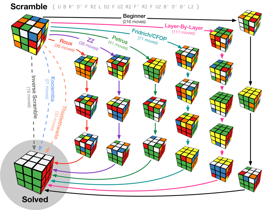
Knowing the mechanics of the cube from the previous post is the foundation. Now the question is how to actually solve it – and more specifically, what different solving strategies exist, what they optimize for, and why those differences matter. This is not a step-by-step tutorial. It is an overview of the main methods with enough depth to understand the tradeoffs, which is what you need before the mathematics and algorithmic approaches in the next posts make full sense.

Human solving methods are worth studying even if your goal is to build a computer solver, for the same reason that understanding how a problem has been approached manually gives you better intuition about the problem’s structure. Each method below embeds a different set of assumptions about which subproblems to solve first, which tradeoffs to make between move count and algorithmic complexity, and what an efficient solution path looks like.

Layer-by-Layer: Where Most People Start

The Layer-by-Layer method (LBL) is the most common beginner approach. The cube is divided conceptually into three horizontal layers, and each is solved in sequence from bottom to top.

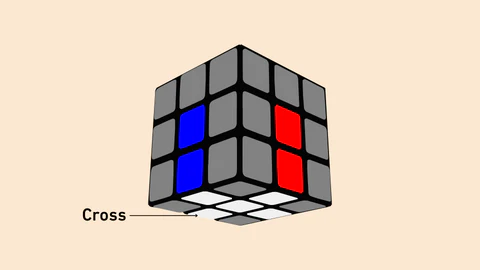
Step one: solve the first layer. This means forming a cross on the bottom face – placing the four bottom-layer edge pieces correctly oriented – and then inserting the four bottom-layer corner pieces.

Step two: solve the middle layer. The four middle-layer edge pieces are inserted one at a time using a standard algorithm that moves them from the top layer into their correct middle positions.

Step three: solve the top layer in two stages. First orient all top-layer pieces so the top face becomes a single color (this is a reduction problem). Then permute them into their correct positions.

LBL is beginner-friendly because each step is isolated. You solve one thing, then the next, and already-solved pieces are not disturbed by subsequent steps. The tradeoff is efficiency: because corners and edges are solved separately in the first layer, and because the top layer takes two distinct steps, the total move count tends to be high – typically 100 to 120 moves for a beginner.

For a software perspective, LBL illustrates the general principle of staged reduction: break the problem into subproblems, solve each without disturbing the previous. This is computationally safe but not optimal, and it maps roughly to how Thistlethwaite’s and Kociemba’s algorithms are structured at a high level, though those are far more sophisticated in execution.

CFOP: The Dominant Speedcubing Method

CFOP stands for Cross, First Two Layers, Orientation of Last Layer, Permutation of Last Layer. It was developed and popularized by Jessica Fridrich, and is the method used by a large majority of competitive speedcubers. I use CFOP myself – intuitive cross and F2L, two-look OLL, one-look PLL.

Cross. The solve begins by solving a cross on one face – typically white by convention, though advanced solvers choose based on inspection. The cross means four edge pieces placed correctly, all aligned with their adjacent center colors, in as few moves as possible. Strong solvers aim to complete the cross in 8 moves or fewer, and they plan it entirely during the 15-second inspection time allowed in competition. A poorly planned cross forces cube rotations and inefficient first pair insertions later, so this step sets the quality of the entire solve.

F2L (First Two Layers). Rather than solving the first-layer corners and then the second-layer edges separately as LBL does, CFOP pairs each corner with its corresponding edge and inserts them together into the correct slot. There are 41 recognized F2L cases, each with known algorithms, but F2L is ideally learned intuitively first – understanding why the pair goes in the way it does, rather than memorizing a move sequence for each case.

This pairing step is the most consequential departure from LBL. By combining two operations that LBL treats separately, CFOP reduces total move count significantly and allows the solver to maintain lookahead – thinking about the next pair while executing the current one. Advanced solvers complete all four F2L pairs with minimal pausing and very few full cube rotations.

OLL (Orientation of Last Layer). Once F2L is done, the top layer has all pieces in their correct layer but not necessarily pointing the right way. OLL fixes this in one step: after a single algorithm, every sticker on the top face points upward. There are 57 distinct OLL cases. Beginners can use a two-look variant (first orient the edges, then the corners) that reduces the algorithm count to 10, at the cost of one extra step.

PLL (Permutation of Last Layer). The top face is now correctly oriented but the pieces around the sides may still be in the wrong positions. PLL permutes them into their correct locations. There are 21 PLL cases. Beginners can use a two-look PLL that requires only 6 algorithms.

Full CFOP requires memorizing 78 algorithms (57 OLL + 21 PLL), plus developing intuitive F2L. In exchange, it enables fast, predictable solve times with a typical move count of 50 to 60 moves for an experienced solver. The structure is rigid enough to be practiced systematically but flexible enough that a skilled solver is constantly making real-time decisions during F2L rather than following a predetermined script.

My own setup: Cubelelo profile for times (unofficial, but still tracked). For 2x2, I use CLL (Corners of the Last Layer), which solves all four last-layer corners in one look using a set of 42 algorithms.

Roux: Block Building Over Algorithm Memorization

Roux was developed by Gilles Roux in 2003. It takes a fundamentally different approach by building blocks rather than solving layers, and it prioritizes move efficiency and ergonomics over rigid structure.

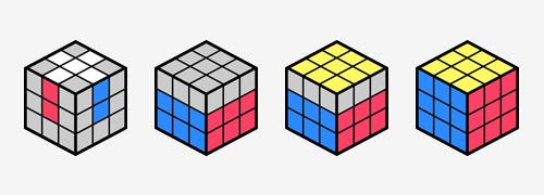
First block. Build a 1x2x3 block on the left side of the cube. This is done intuitively: place three corners and three edges in correct positions and orientations relative to each other, without worrying about anything else.

Second block. Build a 1x2x3 block on the right side. At this point, the left and right blocks are complete, and the only unsolved regions are the top layer and the four middle-slice edges.

CMLL (Corners of the Last Layer). Rather than separating orientation and permutation of the last-layer corners into two steps, Roux handles all four corners simultaneously in one algorithm from a set of 42 CMLL cases. This is equivalent in algorithm count to OLL corners + PLL corners combined, but it is done in a single step.

LSE (Last Six Edges). The final step solves the six remaining edges – four top-layer edges and two center-slice edges – using only M (middle slice) and U (top face) moves. No cube rotations are required. This step can be done intuitively with practice, and it is what gives Roux its character: smooth, low-rotation, ergonomic execution at the end of the solve.

Roux typically produces lower move counts than CFOP (averaging around 45 moves for an expert) and involves fewer cube rotations, which benefits one-handed solving in particular. The tradeoff is that block building is harder to learn systematically than CFOP’s algorithm-based steps. There is no fixed procedure for building the first block – you develop intuition through practice, which takes longer.

ZZ: Edge Orientation First

The ZZ method, created by Zbigniew Zborowski, makes a distinct architectural choice: solve edge orientation before anything else. Once edges are correctly oriented, all remaining steps can be executed using only R, L, and U moves – no F, B, D, or cube rotations required.

EOLine. Orient all 12 edges while simultaneously placing two specific edges (DB and DF) along the bottom. Edge orientation is a binary property – each edge is either correctly oriented (in the sense that it can be placed in its solved position using only R, L, and U moves) or it is not. EOLine sets up the rest of the solve.

F2L. With edges pre-oriented and the two bottom edges in place, the first two layers can be solved using only R, L, and U moves. No cube rotations, no F or B turns, no disruption to the bottom structure. This is ergonomically efficient and produces a very smooth solve once EOLine is handled correctly.

Last layer. Because all edges are oriented, the last layer can be solved with reduced algorithm sets. The most advanced ZZ practitioners use ZBLL (Zborowski-Bruchem Last Layer), which solves the entire last layer in one step from any state. ZBLL requires over 400 algorithms, making it one of the most memorization-heavy approaches in competitive cubing. Most ZZ users start with CFOP-style OLL and PLL, since the edge orientation work in EOLine makes many OLL cases impossible.

ZZ’s main advantage is ergonomics and the low rotation requirement. Its main obstacle is EOLine, which is harder to see quickly than a cross and requires different intuition. Move counts are comparable to CFOP or slightly better.

Petrus: Staged Block Building

The Petrus method, developed by Lars Petrus, uses progressive block expansion rather than layer-by-layer reduction.

Start with a 2x2x2 block in one corner. Expand it to a 2x2x3 block – add one more layer of pieces to the block you already have. At this point, orient the remaining edges (similarly to EOLine in ZZ, this step unlocks efficient moves for the rest of the solve). Then complete the first two layers. Finally, solve the last layer.

Petrus typically produces low move counts and was highly competitive in the early days of speedcubing before CFOP’s infrastructure of algorithms and training resources developed. It is less popular now not because it is worse but because CFOP has a larger community and more developed learning resources.

What These Methods Have in Common

Every method above is a staged reduction strategy. The cube’s full state space is enormous, and no method attacks it directly. Instead, each method constrains the problem progressively: fix some subgroup of pieces, then fix another, then another, until nothing is left to fix.

The methods differ in which subproblems they define, what order they solve them, and how much they exploit structure (like block building or edge pre-orientation) to make later steps cheaper. CFOP is structured and algorithm-heavy, trading memorization cost for speed and predictability. Roux and Petrus rely more on intuitive block building and tend toward lower move counts at the cost of harder-to-systematize learning. ZZ front-loads constraint work (EOLine) to unlock ergonomic efficiency later.

This structure – staged reduction through subgroup constraints – is exactly the framework that Thistlethwaite’s and Kociemba’s algorithms formalize mathematically. The human methods are heuristic approximations of the same underlying idea. Understanding why a human solver orients edges before inserting corners makes it much easier to understand why a computer algorithm might maintain edge orientation as an invariant across its search phases.

The next post goes into the mathematics: how the cube’s state space is counted, what group theory says about the structure of moves, and what properties of the cube group make efficient algorithmic solving possible.