What is SLAM? And Why It's the Brain of Mobile Robots
A mobile robot navigating an unknown environment faces two problems that are coupled in a way that makes each one unsolvable without the other. To localize itself, the robot needs a map to compare its sensor readings against. To build a map, it needs to know where it is so that it can correctly register new observations into the map. Neither the map nor the pose is known at the start. Both must be estimated simultaneously from the same stream of sensor data. This is the SLAM problem: Simultaneous Localization and Mapping.
The coupling is what makes SLAM non-trivial. If the robot’s trajectory were known exactly, building a map would be straightforward: sensor observations would be projected into the world frame using the known pose and accumulated into a consistent representation. If the map were known exactly, localization would be a standard state estimation problem. The difficulty is that errors in pose estimation cause distortions in the map, and a distorted map causes larger pose estimation errors in subsequent steps. Without mechanisms to detect and correct these accumulated errors, SLAM implementations diverge over time regardless of sensor quality.
Problem Formulation
The formal statement of SLAM requires careful definition of what is being estimated. Let $x_t$ denote the robot’s pose at time $t$, which in 2D is a three-dimensional vector $(x, y, \theta)$ representing position and heading, and in 3D is an element of the Lie group $SE(3)$ representing a full rigid body transformation. Let $m$ denote the map, which may be represented as a set of landmarks with positions, an occupancy grid assigning occupancy probability to a discretized spatial volume, or a continuous implicit surface representation. Let $u_t$ denote the control input applied between time $t-1$ and time $t$, and let $z_t$ denote the sensor observation at time $t$.
The SLAM posterior is the joint distribution over the robot’s trajectory and the map given all observations and controls:
$$ P(x_{1:t}, m \mid z_{1:t}, u_{1:t}) $$This is not a tractable distribution to maintain in closed form for general motion and observation models. The state space of the trajectory alone grows with time, and the joint space of trajectory and map is enormous. Practical SLAM algorithms approximate this posterior in different ways, and the choice of approximation determines the computational complexity, the accuracy, and the types of environments the algorithm handles well.
The Motion and Observation Models
All SLAM algorithms are built on two probabilistic models. The motion model describes how the robot’s pose evolves as a function of control inputs and process noise:
$$ x_t = f(x_{t-1}, u_t) + w_t $$where $f$ is the kinematic motion function and $w_t$ is process noise, typically modeled as zero-mean Gaussian with covariance $Q_t$. For a differential drive robot with wheel encoders, $f$ integrates the odometry, and the noise model accounts for wheel slip, encoder quantization, and integration drift. Odometry noise accumulates unboundedly over time. A robot that drives in a large loop and returns to its starting position will, using odometry alone, estimate that its final position is displaced from its starting position by an error that grows with the total distance traveled.
The observation model describes the distribution over sensor measurements given the robot’s pose and the map:
$$ z_t = h(x_t, m) + v_t $$where $h$ is the observation function and $v_t$ is observation noise with covariance $R_t$. For a 2D LiDAR, $h$ computes the expected range measurements to the nearest obstacles for each beam direction given the known map and the robot’s pose. The discrepancy between predicted and actual measurements is used to update the pose estimate. The observation model is the mechanism by which sensor data reduces uncertainty; without it, uncertainty grows with each motion step due to process noise and is never corrected.
The Bayesian filter formulation combines these models into a recursive update. The prediction step propagates the current belief through the motion model, increasing uncertainty. The update step incorporates the new sensor observation, reducing uncertainty in directions that the sensor can observe. SLAM is a Bayesian filtering problem over the joint space of pose and map, which is what makes the computational challenge so severe.
Extended Kalman Filter SLAM
The oldest and most analytically tractable SLAM formulation maintains the joint posterior as a Gaussian distribution over the robot’s pose and the positions of a set of point landmarks. The state vector is:
$$ \mu = \begin{bmatrix} x \\ m_1 \\ m_2 \\ \vdots \\ m_n \end{bmatrix}, \quad \Sigma = \text{full covariance matrix} $$where $x$ is the three-dimensional pose (in 2D) and $m_i$ is the two-dimensional position of the $i$-th landmark. The covariance matrix $\Sigma$ has dimension $(3 + 2n) \times (3 + 2n)$ and encodes the uncertainty in each quantity and the correlations between them.
The correlations are important and easily overlooked. When a landmark is first observed, its estimated position is uncertain because the robot’s pose is uncertain. That uncertainty in landmark position is correlated with the robot’s pose uncertainty because both stem from the same source: accumulated odometry error. As the robot continues to observe the landmark from different locations, the correlation between the robot’s pose and the landmark position becomes a mechanism for updating both estimates together. A loop closure, where the robot recognizes a previously mapped landmark from a new viewpoint, is a highly informative observation precisely because it constrains the robot’s pose relative to a point that was mapped earlier under a different accumulated error.
EKF-SLAM propagates this covariance through the nonlinear motion and observation functions using first-order Taylor expansion, which is the extended Kalman filter. The computational cost of the covariance update is $O(n^2)$ per timestep, where $n$ is the number of landmarks, because updating one landmark’s position in response to a new observation requires updating its correlation with every other landmark in the map. For small environments with tens to hundreds of landmarks, this is feasible. For large environments with thousands of landmarks, the $O(n^2)$ scaling becomes prohibitive.
EKF-SLAM also assumes Gaussian uncertainty, which is appropriate for unimodal distributions but fails when the robot’s pose is genuinely ambiguous. In an environment with repeated structure, such as a corridor with evenly spaced identical doorways, the robot may be in one of several distinct locations consistent with the current observation. A single Gaussian cannot represent this multimodal distribution; it can only represent a single probability peak. EKF-SLAM in such environments produces overconfident estimates that converge on the wrong mode.
Particle Filter SLAM and FastSLAM
The FastSLAM family of algorithms addresses the multimodality problem by using a particle filter to represent the distribution over robot trajectories, while maintaining a separate Gaussian estimate of each landmark’s position conditioned on each particle’s trajectory.
The factorization that makes this work is:
$$ P(x_{1:t}, m \mid z_{1:t}, u_{1:t}) = P(x_{1:t} \mid z_{1:t}, u_{1:t}) \cdot P(m \mid x_{1:t}, z_{1:t}) $$The trajectory distribution $P(x_{1:t} \mid z_{1:t}, u_{1:t})$ is represented by a set of particles, each of which is a sampled trajectory through the environment. The map distribution conditioned on each trajectory $P(m \mid x_{1:t}, z_{1:t})$ decomposes into independent per-landmark distributions when the observation model is such that each observation involves only one landmark. Given a known trajectory, the landmarks are conditionally independent of each other. This means each particle maintains $n$ independent Gaussian landmark estimates rather than a joint covariance over all landmarks, reducing the per-particle storage from $O(n^2)$ to $O(n)$.
A particle represents one hypothesis about the robot’s trajectory. Particles that are consistent with the observations receive higher weights and are more likely to be resampled. The result is a population of particles that concentrates on trajectories that are consistent with the full history of observations. Multimodal distributions are handled naturally because multiple distinct hypotheses can coexist as separate particles.
The weakness of particle filters is that the number of particles required to maintain an accurate approximation grows with the dimensionality of the state space. For 2D navigation, a few hundred to a few thousand particles are often sufficient. For 3D navigation with full $SE(3)$ pose uncertainty, the particle count needed for adequate coverage of the distribution is much larger, and the computational cost grows proportionally.
Graph-Based SLAM
The most widely used SLAM formulation in current systems represents the problem as a pose graph and solves it as a nonlinear least squares optimization. Nodes in the graph represent robot poses at selected timesteps (keyframes) and possibly landmark positions. Edges represent constraints derived from sensor observations: a constraint between two poses says that the robot’s relative transformation between those two poses, as estimated from the sensor data observed between them, is $z_{ij}$ with information matrix $\Omega_{ij}$.
The optimization finds the configuration of poses and landmarks that minimizes the total squared error across all constraints:
$$ x^* = \arg \min_x \sum_{(i,j) \in \mathcal{E}} \| z_{ij} - h(x_i, x_j) \|^2_{\Omega_{ij}} $$where the norm $\| \cdot \|^2_{\Omega}$ is the Mahalanobis norm weighted by the information matrix, and $h(x_i, x_j)$ is the predicted relative measurement between poses $x_i$ and $x_j$.
This formulation separates the front-end, which processes raw sensor data to extract constraints, from the back-end, which solves the optimization. The front-end is sensor and environment specific: it handles feature extraction, data association (determining which observations correspond to which landmarks or previously visited poses), and constraint construction. The back-end is a general nonlinear least squares solver, and efficient solvers like g2o and Ceres exploit the sparse structure of the pose graph to achieve efficient optimization.
The key observation is that in a pose graph built from sequential motion, the information matrix of the full system is sparse: each new constraint adds edges only between nearby nodes or between a current node and a previously visited one. Sparse matrix methods allow the full optimization to be solved in time proportional to the number of edges rather than the cube of the number of nodes, making graph-based SLAM scalable to large environments.
Loop Closure
Loop closure is the mechanism by which accumulated drift is corrected. When a robot travels through a large environment and returns to a previously visited location, the observations from the current position should match the map built from the earlier visit. If the match is detected, the constraint it provides, a relative transformation between the current pose and the earlier pose with low uncertainty, adds a long-range edge to the pose graph that is inconsistent with the trajectory predicted by odometry alone. Optimizing the graph over all constraints, including this new loop closure constraint, distributes the accumulated error across the entire loop, typically reducing the total map distortion.
Without loop closure, the map error grows monotonically with distance traveled. A robot that maps a 100-meter corridor accumulates enough odometry drift that the two ends of the corridor, which should match, are displaced by meters in the estimated map. With loop closure, that error is corrected at the moment the robot recognizes the match.
The detection of loop closures is the most fragile part of the SLAM pipeline. It requires recognizing that the current sensor data was observed before, from a different position with potentially different viewpoint, lighting, and dynamic objects. For LiDAR-based SLAM, scan matching algorithms can compare point cloud descriptors across large databases of prior scans. For camera-based SLAM, place recognition uses visual features or learned embeddings to identify revisited locations. Both approaches produce false positives, cases where the recognition system incorrectly identifies two distinct locations as the same, which adds incorrect constraints to the pose graph and can distort the map catastrophically. Robust loop closure detection requires a verification step that checks geometric consistency between the proposed correspondence and the existing map before the constraint is added.
Pose Representation on Lie Groups
For 3D SLAM, the robot’s pose is an element of the Lie group $SE(3)$, the group of rigid body transformations in three dimensions:
$$ T = \begin{bmatrix} R & t \\ 0 & 1 \end{bmatrix} \in SE(3) $$where $R \in SO(3)$ is a rotation matrix satisfying $R^T R = I$ and $\det(R) = 1$, and $t \in \mathbb{R}^3$ is a translation vector. Representing pose as a $4 \times 4$ matrix imposes the $SO(3)$ constraint on the rotation, which means that naive optimization over the 16 elements of the matrix would require enforcing the constraint explicitly.
Modern SLAM back-ends use manifold-aware optimization, where incremental updates to the pose are represented in the Lie algebra $\mathfrak{se}(3)$, a six-dimensional vector space that serves as the local linearization of $SE(3)$ at any given point. The exponential map $\exp: \mathfrak{se}(3) \to SE(3)$ maps tangent vectors to group elements, allowing incremental updates to be applied as $T \leftarrow T \cdot \exp(\delta\xi)$ where $\delta\xi$ is the six-dimensional update computed by the optimizer. This ensures that the rotation component remains in $SO(3)$ after each update without explicit constraint enforcement.
The practical consequence is that the Jacobians computed during optimization are with respect to the Lie algebra coordinates rather than the matrix elements, and the linearization is accurate to first order in the neighborhood of each iterate. GTSAM, g2o, and Ceres all implement this manifold-aware update pattern for $SE(3)$ and $SO(3)$ poses.
Sensor Modalities
The specific sensor determines what the observation model looks like and what kinds of environments the SLAM system handles well.
2D LiDAR produces range measurements at a fixed set of angles in a horizontal plane. It is accurate, fast, and produces dense measurements. The observation model is well-understood, and scan matching algorithms for 2D LiDAR are mature. The limitation is the dimensionality: a 2D LiDAR cannot observe a 3D environment, and environments that look similar at a fixed height (long corridors, large open spaces) provide weak constraints for localization.
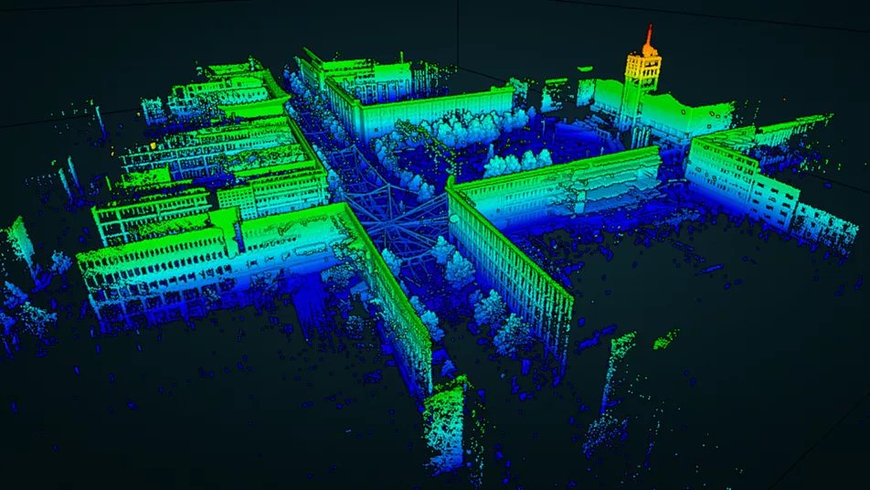
3D LiDAR produces point clouds covering a three-dimensional volume around the sensor. It provides richer constraints and works in environments where 2D LiDAR fails. The data rate is much higher (millions of points per second for rotating scanners), which requires efficient data structures for storage and matching.
Cameras provide dense visual information that LiDAR does not capture: texture, color, and the semantic content of the scene. Visual SLAM extracts features from images (corners, blobs, or learned descriptors), matches them across frames, and estimates the camera motion from the feature correspondences. The observation model is the reprojection function that projects a 3D landmark into the image plane given the camera pose and intrinsic parameters. The limitation is sensitivity to illumination changes, featureless environments, and motion blur.
Inertial measurement units provide high-rate measurements of linear acceleration and angular velocity. IMU measurements can be integrated to propagate pose at high frequency between camera or LiDAR updates. IMU integration drift, especially in rotation, is large over seconds to minutes, but over the short intervals between camera frames it provides useful constraints that improve both the accuracy and the robustness of visual or LiDAR odometry. IMU-visual fusion is the basis of all current state-of-the-art visual-inertial SLAM systems.
Where SLAM Is and Where It Is Going
The core mathematical structure of SLAM has been understood since the late 1980s and early 1990s. The EKF-SLAM formulation dates to Smith, Self, and Cheeseman (1986) and Moutarlier and Chatila (1989). The sparse graph formulation that dominates current practice was established by Lu and Milios (1997) and extended through the 2000s as efficient sparse solvers became available. What has changed is the engineering: more capable sensors, faster processors, better feature representations, and large-scale deployment in products like autonomous vehicles, robot vacuum cleaners, and AR headsets have refined the implementations substantially.
The open problems are at the boundary between geometry and semantics. Standard SLAM builds geometric maps: collections of points, surfaces, or occupancy cells. A robot using such a map can localize within it but cannot reason about what the objects in the environment are, which ones can be moved, or which ones are relevant to a task. Semantic SLAM adds object-level understanding to the geometric map, labeling parts of the map with object categories and using semantic consistency as an additional constraint during loop closure and localization. This is an active research area, and current systems handle it reasonably well in structured indoor environments with known object categories but do not generalize robustly to arbitrary environments.
Dynamic objects are handled poorly by standard SLAM, which assumes a static world. Sensor measurements that do not correspond to static structure are treated as outliers and discarded, but in environments with significant dynamic content (pedestrians, moving vehicles, other robots) the outlier rate becomes high enough to degrade localization. Dynamic SLAM methods attempt to track moving objects explicitly and factor them out of the static map estimation, but this adds substantial complexity and is an unsolved problem for cluttered, high-dynamic environments.
Lifelong SLAM, where the robot must maintain a map over months or years as the environment changes, is a further open problem. Static maps become stale as furniture is moved, buildings are renovated, and seasonal changes alter outdoor appearance. Efficient map update strategies that can integrate new observations while forgetting obsolete ones are necessary for long-term deployment but are not well-standardized across systems.