ImProVe: Image Processing using Verilog

Project Overview

ImProVe is an initiative to implement core image processing algorithms using Verilog. It aims to achieve real-time performance for advanced applications in fields like robotics, medical imaging, and computer vision.

Motivation

On November 26, 2024, while preparing for my Verilog elective exam, I needed to scan and rotate images of handwritten notes. That’s when I thought:

“Can image rotation be implemented using Verilog?”

This led me to experiment with basic transformations like rotation, cropping, translation, and shearing. As I explored further, I expanded the scope to include edge detection methods (Prewitt, Sobel, Kirsch Compass, Robinson Compass, and Canny) and noise reduction techniques (median, Gaussian, and box filters).

Initially, I wasn’t familiar with the mathematical foundations of these techniques, so I learned them as I implemented each one. The project started as RoVer – Rotation using Verilog, focusing solely on image rotation. Over time, it evolved beyond simple transformations, leading to the creation of ImProVe – Image Processing Using Verilog.

Aim

The goal of this project is simple yet ambitious: Build a set of foundational image processing blocks using Verilog that can be deployed on hardware for real-world applications.

These blocks will enable practical applications such as label detection, document scanning, object recognition, and more, making real-life automation and AI-driven vision tasks possible.

THE Challenge

The project isn’t just about implementing these techniques—it’s about making them synthesizable for hardware. Currently, there are many simulation constructs that aren’t FPGA-friendly. Fixing this is a big part of the journey.

Features

ImProVe supports a wide array of image processing functionalities categorized into multiple domains:

01 Edge Detection and Feature Extraction

• ✅ Sobel Operator: Detects edges by computing gradients in horizontal and vertical directions
• ✅ Prewitt Operator: Similar to Sobel but uses different kernel values
• ✅ Roberts Cross Operator: Uses a 2x2 kernel for edge detection
• ✅ Robinson Compass Operator: Uses eight directional masks to detect edges with specific orientation sensitivity
• ✅ Kirsch Compass Operator: Detects edges by applying a set of 3x3 masks to enhance edges in various directions
• ✅ Laplacian Operator: Captures edges by computing the second derivative of the image, highlighting regions of rapid intensity change
• ✅ Laplacian of Gaussian (LoG): Combines edge detection with noise reduction
• ✅ Canny Edge Detection: Advanced edge detection using gradients, non-maximum suppression, and thresholding
• ✅ Emboss Filter: Applies a convolution kernel to highlight edges and create a 3D relief effect
• ✅ Moravec Corner Detection: Detects corners by evaluating changes in intensity in various directions using a 3x3 window
• 🔲 Harris Corner Detection: Identifies corners by analyzing intensity gradients

02 Noise Reduction and Smoothing

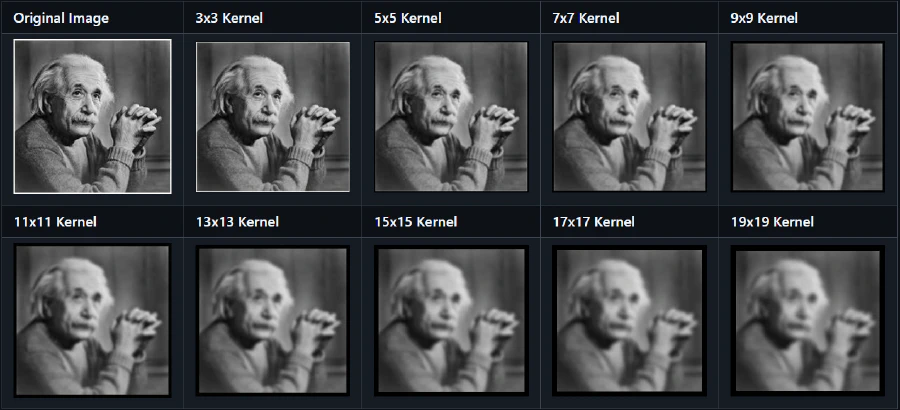
• ✅ Gaussian Blur: Smoothens and reduces noise using a Gaussian kernel
• ✅ Median Filter: Replaces each pixel with the median of its neighborhood to remove Noise
• ✅ Box Filter (Mean Filter): Averages pixel values within a window for Smoothing
• ✅ Bilateral Filter: Preserves edges while reducing noise by combining spatial and intensity information

03 Thresholding and Binarization

• ✅ Global Thresholding: Converts grayscale images to binary using a fixed thresholding
• ✅ Adaptive Thresholding: Dynamically computes thresholds based on local Intensity
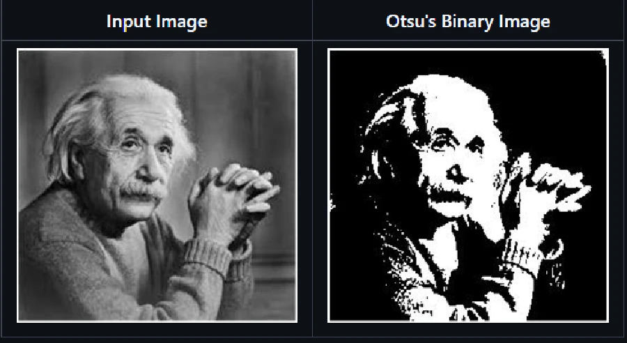
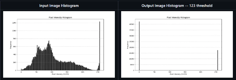
• ✅ Otsu’s Method: Automatically finds the optimal threshold for binarization
• ✅ Color Thresholding: Applies thresholding on color spaces (e g , RGB, HSV, LAB) to segment specific color ranges

04 Morphological Operations

• 🔲 Erosion: Shrinks objects by removing pixels on boundaries
• 🔲 Dilation: Grows objects by adding pixels to boundaries
• 🔲 Opening: Removes noise using erosion followed by dilation
• 🔲 Closing: Fills small holes using dilation followed by erosion
• 🔲 Boundary Extraction: Extracts object boundaries from binary images

05 Filtering and Transformations

• 🔲 Convolution Filtering: Applies custom kernels for sharpening, blurring, and edge enhancement
• 🔲 High-Pass Filtering: Enhances edges and fine details
• 🔲 Low-Pass Filtering: Removes high-frequency noise for smoother images
• 🔲 Fourier Transform: Converts spatial data to frequency domain for filtering
• 🔲 Discrete Cosine Transform (DCT): Used for image compression (e g , JPEG)
• 🔲 Wavelet Transform: Decomposes images for multiscale analysis

06 Geometric Transformations

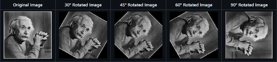
• ✅ Rotation: Rotates the image by a given angle
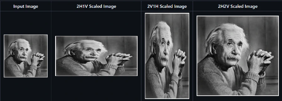
• ✅ Scaling: Resizes the image while preserving aspect ratio
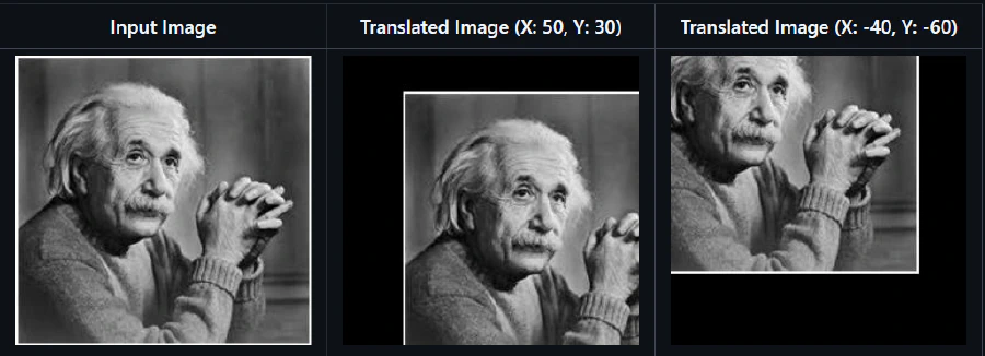
• ✅ Translation: Shifts the image position
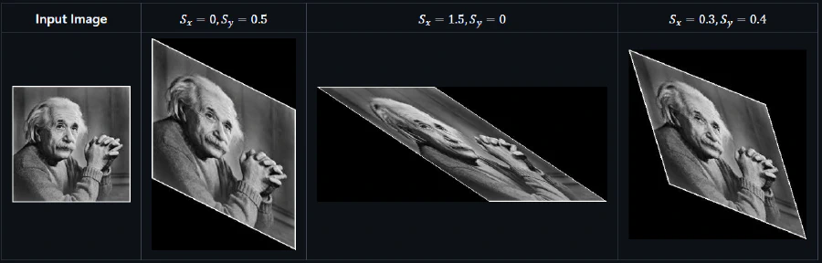
• ✅ Shearing: Distorts the image by shifting rows or columns
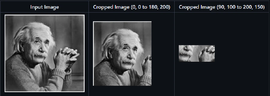
• ✅ Cropping: Extracts a rectangular region from the image
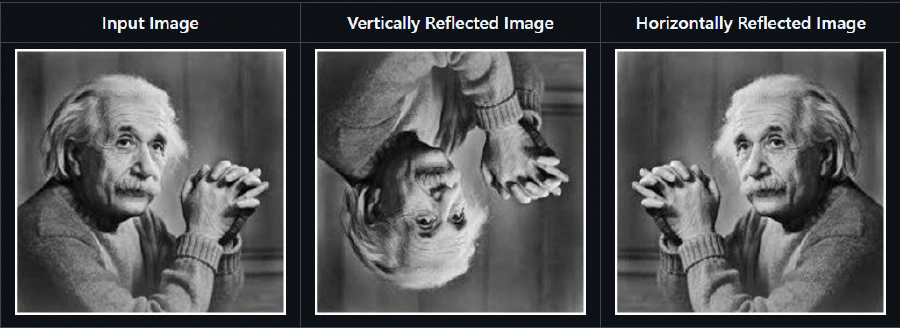
• ✅ Reflection: Flips the image across a specified axis (horizontal, vertical, or diagonal)
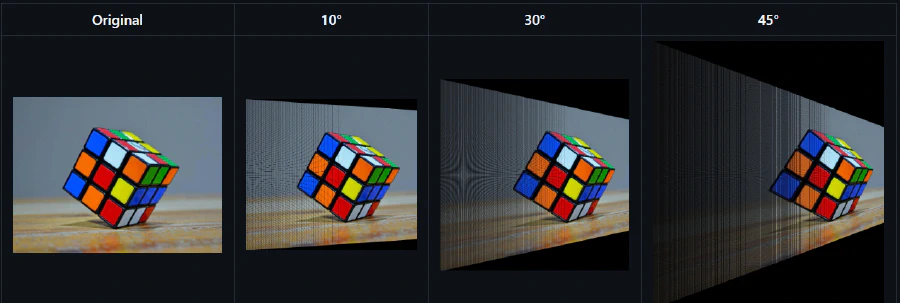
• ✅ 3D Perspective Transformation: Applies a projective transformation that distorts the image to simulate depth
• 🔲 Affine Transformations: Combines translation, scaling, rotation, and shearing

07 Histogram-Based Processing

• 🔲 Histogram Equalization: Enhances image contrast by redistributing pixel intensity
• 🔲 CLAHE: Locally enhances contrast in small regions
• 🔲 Histogram Matching: Matches the histogram of one image to another

08 Texture Analysis

• 🔲 Gabor Filters: Extracts texture features using orientation-sensitive filters
• 🔲 Local Binary Patterns (LBP): Captures texture by comparing neighboring pixel intensities
• 🔲 Haralick Features: Computes texture features from the gray-level co-occurrence matrix

09 Color and Intensity Transformations

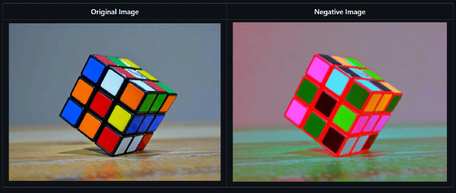
• ✅ Negative Transformation: Converts an image to its negative by replacing each pixel value ( R ) with ( 255 - R )
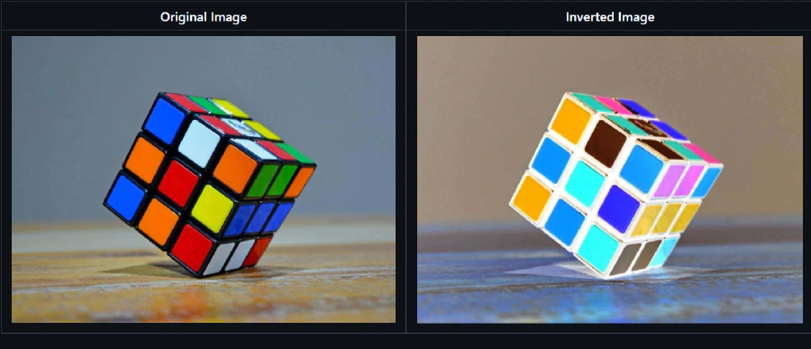
• ✅ Inversion: Converts an image to its negative by inverting pixel values
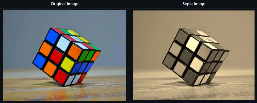
• ✅ Sepia Effect: Applies a warm brown tone to an image for a vintage look
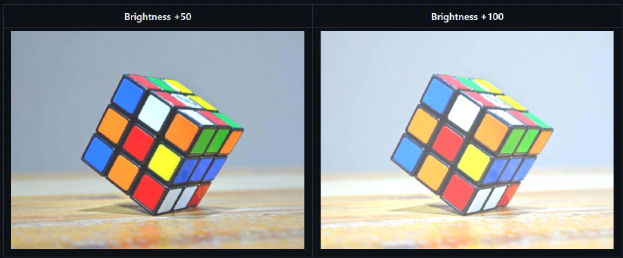
• ✅ Brightness Adjustment: Modifies image brightness by increasing or decreasing pixel intensity
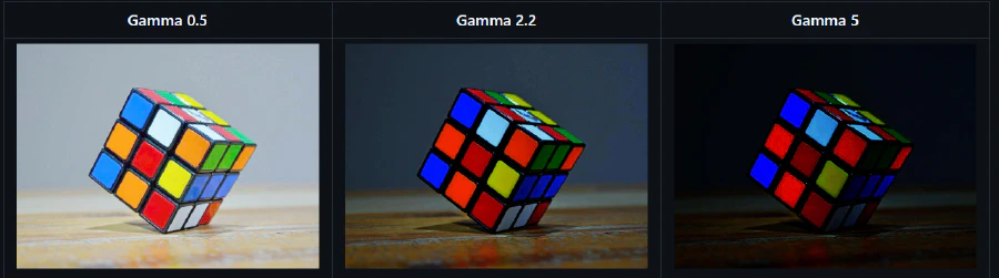
• ✅ Gamma Correction: Adjusts brightness using a gamma function
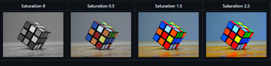
• ✅ Saturation Adjustment: Enhances or reduces color intensity using a scaling factor
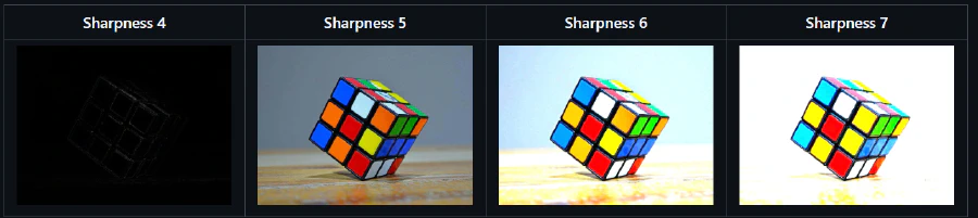
• ✅ Sharpness Enhancement: Increases edge contrast to make the image appear clearer
• 🔲 Logarithmic Transformation: Expands dark regions in an image
• 🔲 Power-Law Transformation: Enhances image intensity using power-law curves

10 Object Detection and Segmentation

• 🔲 Template Matching: Detects objects by correlating with a template
• 🔲 Connected Component Labeling: Labels connected regions in binary images
• 🔲 Watershed Algorithm: Segments images based on intensity gradients
• 🔲 Active Contour (Snake Algorithm): Iteratively detects object boundaries
• 🔲 Region Growing: Segments images based on pixel similarity

11 Optical Flow and Motion Analysis

• 🔲 Lucas-Kanade Method: Estimates optical flow for motion detection
• 🔲 Horn-Schunck Method: Computes dense optical flow for pixel-level motion analysis
• 🔲 Frame Differencing: Detects motion by subtracting consecutive frames

12 Image Restoration

• 🔲 Deconvolution: Restores blurred images caused by motion or defocus
• 🔲 Wiener Filter: Reduces noise while preserving image details
• 🔲 Inpainting: Fills missing or corrupted image regions

13 Compression Algorithms

• 🔲 Run-Length Encoding (RLE): Compresses binary or grayscale images
• 🔲 Huffman Encoding: Compresses data using variable-length codes
• 🔲 JPEG Compression: Combines DCT, quantization, and Huffman encoding for image compression

More to Come :)

TODO

• Ensure the code is synthesizable by removing all non-synthesizable constructs.
• Use CORDIC to eliminate functions like $cos, $sin, $exp, $sqrt, and other complex mathematical operations.
• For constructs related to file I/O and read/write operations, use BRAM or RAM memory to store the input image in pixels.
• The output image data for all three channels should be connected to a VGA display via a communication bus like PCIe or AXI.
• Optimize the solution for performance and resource efficiency.

Currently working on CORDIC: CORDIC Algorithm in Verilog

Currently working on OCR using Verilog as well, building a neural network from scratch for MNIST number recognition

Tools and Technologies

• Icarus Verilog 12 0: Core HDL used to implement all image processing algorithms
• Python 3 12 1: For preprocessing image data into a format compatible with verilog

Applications IRL

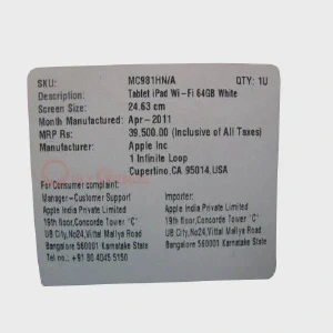
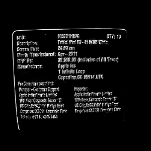
Label-Detection

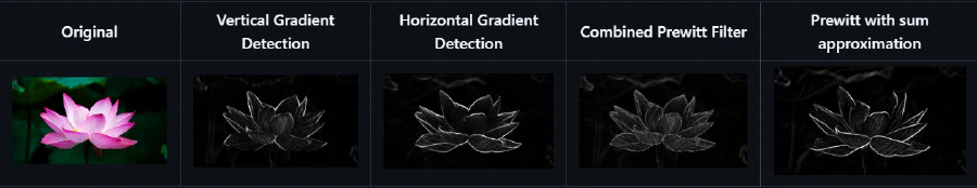
• Label detection was implemented using the Prewitt operator for edge detection. The process begins by splitting the image into three separate RGB channels using Python. Next, the luminance formula (NTSC) is applied to obtain a grayscale image.

• If the image is too noisy or requires preprocessing, Gaussian blur and morphological operations are applied to refine the grayscale image before edge detection.

• Edge detection algorithms are then used to identify strong edges. From these edges, the flood-fill algorithm is applied to detect the largest possible contour. A bounding rectangle is drawn in the red channel to enclose this contour, which is then superimposed on the original image for clear label detection.

• This entire process is executed in Verilog using text files for data handling. Python is then used for visualization to generate the final output.

*For more details

Original Image	After Vertical Prewitt	After Horizontal Prewitt	After Full Prewitt

Original Image	After Full Prewitt	Binary Box	Overlayed Image with Box

Original Image	After Full Prewitt	Binary Box	Overlayed Image with Box

Document Scanner

• The initial steps of the document scanning process are similar to label detection, with Canny edge detection being the preferred method for stronger edge identification.

• After detecting edges, instead of directly superimposing a bounding rectangle, the boundary-fill algorithm is used to fill the detected region with binary 1s (255). A Boolean operation is then applied to remove irrelevant parts of the image that do not contain the document.

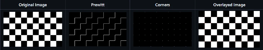
• Next, corner detection is performed using the Moravec operator (as Harris is computationally expensive). Once the corners are identified, Bresenham’s algorithm is used to draw lines connecting them, forming a quadrilateral around the document.

• This quadrilateral is then mapped to a rectangle using homogeneous perspective transformation, followed by shearing and scaling operations if needed to refine the final output.

OTW [Stuck at Bresenham’s algorithm implementation]

Stereo Vision

• The process begins by converting the input stereo image pair from RGB to grayscale. Using the camera parameters, a disparity map is computed to determine the pixel shifts between the left and right images. This disparity information is then used to generate a depth map, which represents the distance of objects in the scene.

• Both the disparity and depth map calculations are implemented entirely in Verilog, using text files for intermediate data storage and processing. Once the depth information is obtained, Python is used to continue the 3D reconstruction process, where the depth map is converted into a point cloud or a 3D mesh representation for visualization.

OTW [Accuracy of disparity and depth maps is low]

MNIST Digit Detection [NeVer ∩ ImProVeD]

• I implemented a simple neural network from scratch in Google Colab without using TensorFlow or Keras, relying solely on NumPy for numerical computations, Pandas for data handling, and Matplotlib for visualization. The dataset used was sample_data/mnist_train_small.csv, containing handwritten digit images in a flattened 784-pixel format. Data preprocessing involved normalizing pixel values (dividing by 255) and splitting it into a training set and a development set, with the first 1000 samples reserved for development and the rest for training. Labels (digits 0-9) were stored separately, and data was shuffled before training to ensure randomness.

• The neural network consists of an input layer (784 neurons), a hidden layer (128 neurons, ReLU activation), and an output layer (10 neurons, softmax activation). Model parameters (weights and biases) were initialized randomly and updated using gradient descent over 500 iterations with a learning rate of 0.1. Training involved forward propagation to compute activations and backpropagation to update parameters. Accuracy was printed every 10 iterations. To make the trained model compatible with Verilog, weights and biases were scaled by 10,000 and saved as integer values in text files (W1.txt, b1.txt, etc.), preventing floating-point multiplication in hardware. These parameters were later reloaded for predictions on new images, verifying model accuracy on the development set before deployment in Verilog for real-time digit classification.

• The model, trained on sample_data/mnist_train_small.csv, achieved over 90% accuracy. It generates W1, W2, b1, and b2 text files containing shape information. The trained parameters are used in Verilog to predict digits from an input image stored in input_vector.txt, which consists of 784 space-separated integers. The predicted output is displayed in the terminal using $display. The original CSV file was converted into a space-separated text format where each line contains a digit followed by 784 pixel values (785 total). During prediction, the first value (label) is removed to test if the model correctly classifies the input image.

• The Verilog module implements a neural network to classify handwritten digits from the MNIST dataset. It comprises an input layer (784 neurons), hidden layer (128 neurons), and output layer (10 neurons). The module reads pre-trained weights and biases from text files (W1.txt, b1.txt, W2.txt, b2.txt) along with an input vector from input_vector.txt. Input values are normalized by dividing by 255.0, while weights and biases are scaled using a factor of 10,000. The hidden layer performs a fully connected transformation (W1 * input + b1) followed by ReLU activation. The output layer computes another weighted sum (W2 * hidden + b2) but does not apply softmax; instead, the predicted digit is determined by selecting the index of the highest output value.

• The file reading process ensures proper loading of weights, biases, and input values before computation begins. Forward propagation occurs sequentially, with an initial delay for data loading. After computing activations in both layers, the module iterates through the output layer to identify the highest value, representing the predicted class. The classification result is then displayed. This hardware implementation streamlines neural network inference by eliminating complex activation functions like softmax while preserving classification accuracy through maximum output activation.

• In newer versions of the code, the text files are converted into synthesizable memory blocks using Python scripts. These scripts store weights and biases in register modules, which are finally instantiated in the top-level module. The image data is also handled in a similar way.

• Only the $display statement, $finish, and the real datatype in the final top-level module are non-synthesizable constructs. These can be eliminated by directing the predicted output to a seven-segment display using case statements [Moved these constructs to the testbench in later versions for a cleaner top module; currently working with Q24.8 as a replacement for the real datatype].

• I am currently working on replacing the training process with a Verilog-based implementation, aiming for a fully synthesizable neural network.

This approach can pave a new way for POC, where text files are converted into register modules using Python scripts to automate the process. A top-level module can then connect all the generated modules, and the testbench can include $fopen, etc., to write the output text files. The testbench instantiates the top-level module, ensuring that all files are synthesizable.

OCR: Optical Character Recognition

This model is trained on the EMNIST ByClass dataset (source), which contains 62 classes (digits 0-9, uppercase letters A-Z, and lowercase letters a-z). The dataset is preprocessed by converting it into a CSV format, normalizing pixel values, reducing dimensions, and shuffling before training.

The neural network consists of multiple layers:

• Input layer: 784 neurons
• First hidden layer: 256 neurons (W1: 256×784, b1: 256×1)
• Second hidden layer: 128 neurons (W2: 128×256, b2: 128×1)
• Output layer: 62 neurons (W3: 62×128, b3: 62×1)

Training is done using forward propagation, computing activations at each layer using matrix multiplications and ReLU activations for hidden layers. Backpropagation is used to update weights using the gradient of the loss function. The dataset is shuffled to improve generalization, and weights (W1, W2, W3) and biases (b1, b2, b3) are updated iteratively until convergence. The model is trained over multiple epochs using stochastic gradient descent (SGD) and Adam’s Optimiser.

To make the trained model compatible with hardware, weights and biases are scaled by 10,000 and stored as integers in text files (W1.txt, b1.txt, etc.), since Verilog does not support floating-point arithmetic.

Inference in Verilog follows a similar process but supports extra layers and classes. Input images are read from input_vector.txt and normalized. Weights and biases are loaded from text files. The computation follows:

• hidden1 = ReLU(W1 * input + b1)
• hidden2 = ReLU(W2 * hidden1 + b2)
• output = W3 * hidden2 + b3

The index of the maximum output value determines the predicted character, which is mapped to "0123456789ABCDEFGHIJKLMNOPQRSTUVWXYZabcdefghijklmnopqrstuvwxyz" and displayed using $display.

The video demonstrates that draw.py allows us to draw anything on a square canvas. At the end, it applies grayscale, inverts the image, compresses it to a 28×28 resolution, and saves it as drawing.jpg. Then, img2bin.py converts this image into a 2D array of pixels (a 28×28 matrix) and saves it in mnist_single_no.txt.

Next, arr2row.py flattens the 2D array into a 1D array (a row of 784 values) and stores it in input_vector.txt. This file is then used to create image_memory.v with memloader_from_inp_vec.py, which generates a memory module for storing the image.

Following this, wtbs_loader.py creates six different memory modules from W1, W2, W3, b1, b2, and b3 text files, generating corresponding files such as W1_memory.v, and so on.

All these components are instantiated in the top module emnist_with_tb.v, along with a testbench (emnist_nn_tb.v). This setup ultimately predicts the drawn character. In the demo, I showcased the characters “H,” “f,” and “7”—each representing a different subclass from the 62 available classes (uppercase letters, lowercase letters, and numbers).

Additionally, I developed a coarse-grained pipelined fully connected neural network using Finite State Machine (FSM) and integrated Softmax with a Taylor series approximation to improve computational efficiency

Important Links and Resources

Digital Image Processing

• GeeksforGeeks: Digital Image Processing Tutorial
• YouTube: Digital Image Processing Introduction
• YouTube Live: Advanced Digital Image Processing Concepts

Mathematics for Engineering and Computing

• YouTube: Building a neural network FROM SCRATCH
• YouTube: I Built a Neural Network from Scratch
• YouTube: Linear Algebra – Essence of Linear Algebra (Playlist)

Verilog

• Guide to Verilog File I/O and File Handling
• Official Icarus Verilog Documentation
• NPTEL Lectures

CORDIC Algorithm Resources

• IEEE Xplore: Hardware Implementation of a Math Module Based on the CORDIC Algorithm Using FPGA
• CORDIC Algorithm and Its Applications in DSP (NITR Thesis)
• CORDIC for Dummies (Introductory Guide)
• STMicroelectronics: Using the CORDIC for Mathematical Functions on STM32 MCUs
• Square Root Calculation Using CORDIC In System Verilog

Datasets

• MNIST Dataset: 0-9 Handwritten Numbers
• EMNIST Dataset: Extended MNIST with Alphabet Support
• Standard OCR Dataset: Various Images of Characters in Different Fonts

Contributors

• Jagadeesh mummanajagadeesh97@gmail com

Feel free to contribute by submitting pull requests or feature suggestions!

If interested in working together, do drop a DM or mail 🙂

NOTE

Missing Images:

• Some of the images may be missing due to unforeseen issues. If you notice any missing images, please inform me

Code Structure:

• Not all code snippets follow the same structural order. This is intentional, as some parts are specifically designed to handle their unique mathematical requirements Priority was given to making each individual piece of code functional rather than ensuring the overall scalability of the project

AI Assistance:

• Fair use of AI (e.g., ChatGPT) was employed for syntax suggestions and debugging. Kudos to ChatGPT for its support!

Math Adaptations:

• Not every piece of code adheres strictly to its intended mathematical model. Verilog’s limitations in computational math have necessitated ample adjustments, with liberties taken to ensure functionality.

Feedback & Help:

• Please let me know if you have any suggestions or tips.
• I am in desperate need of help and would greatly appreciate any assistance or advice.

Thank you for your understanding and support!

Selected Image Processing Results

Below are some of the best results from my image processing work. While there are many more images, including all of them here without relevant explanations wouldn’t be meaningful. For a detailed breakdown of the implementation and the mathematical concepts behind each operation, please refer to my repository.

Edge Detection – Prewitt Operator

Corner Detection - Moravec

Noise Reduction – Gaussian Blur

Thresholding – Otsu’s Method

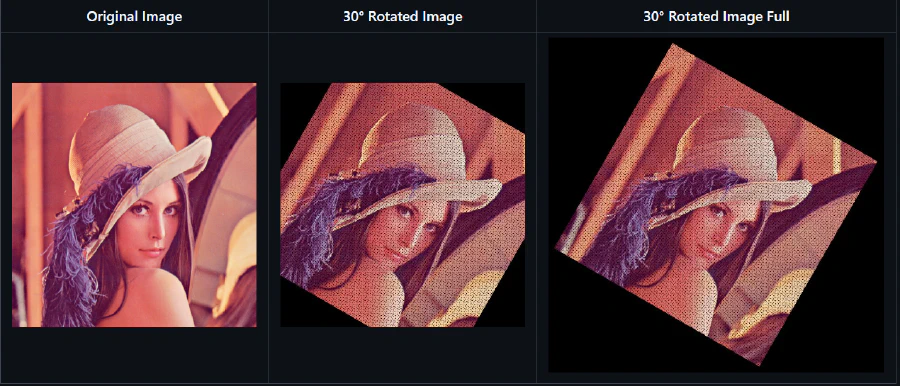
Geometric Transformations

• Rotation with Same Dimensions
  
• Rotation with Diagonal Dimensions
  
• Scaling
  
• Translation
  
• Shearing
  
• Cropping
  
• Reflection (Both Axes)
  
• 3D Homogeneous Perspective Transformation

Color and Intensity Transformations

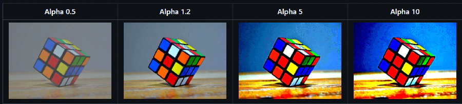
• Gamma Correction
  
• Image Inversion
  
• Sepia Effect
  
• Negative Transformation
  
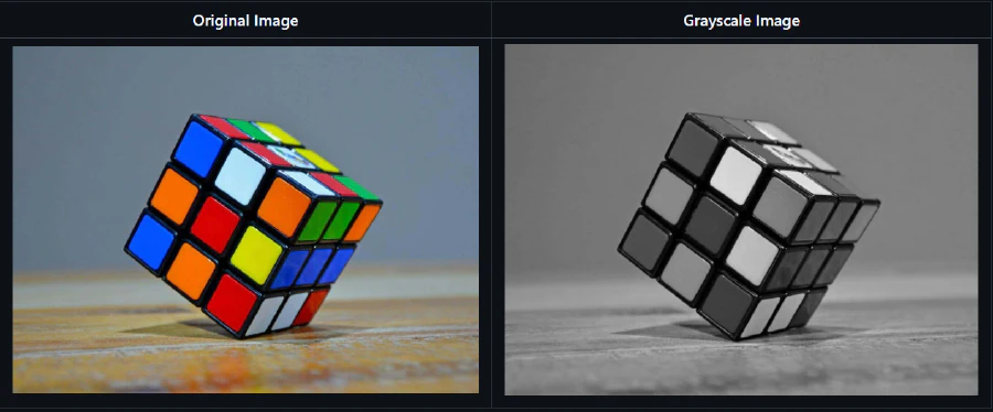
• Grayscale Conversion
  
• Contrast Adjustment
  
• Brightness Adjustment
  
• Saturation Adjustment
  
• Sharpness Enhancement
  

For more insights into the implementation, visit my repository, where I provide a comprehensive explanation of the mathematical foundations behind each operation.

Proof of Concept Proposal: FPGA Implementation of ImProVe

The goal of this proof of concept is to transition ImProVe from a Verilog-based image processing simulation to a fully FPGA-compatible implementation. The current approach, while functional, relies heavily on software-based file I/O, lacks real-time processing capabilities, and does not take advantage of hardware acceleration. This proposal outlines a new FPGA-based workflow that optimizes performance, enables parallel processing, and integrates efficient mathematical computation techniques like CORDIC for trigonometric and square root calculations.

Current Workflow and Its Limitations

The existing implementation is purely simulation-based, using Icarus Verilog without testbenches. Images are pre-processed using Python (NumPy), converted into .hex or .txt files, and then read into Verilog through file I/O functions. After processing, the results are stored in a corresponding output file, converted back into an image, and visually verified or cross-checked with a reference Python implementation.

While this approach enables functional validation, it suffers from several limitations:

• File I/O is slow and does not reflect real-world FPGA-based image processing.
• No hardware optimizations, making it unsuitable for real-time applications.
• No pipelining or parallelism, leading to inefficient processing for large images.
• Mathematical operations (like square root and trigonometric functions) rely on direct computation rather than optimized hardware-friendly methods.

Proposed FPGA-Based Workflow

The FPGA implementation will be designed to replace file-based image processing with a high-speed AXI-based pipeline that processes images in real time. Key improvements include:

CORDIC for Mathematical Computation

Operations like image rotation, edge detection, and geometric transformations require trigonometric functions (sin, cos) and square root calculations. Instead of using costly multipliers or look-up tables, these will be implemented using CORDIC (COordinate Rotation DIgital Computer), which efficiently computes trigonometric functions, logarithms, and square roots in hardware without requiring floating-point arithmetic.

Memory Optimization: DDR for Image Storage, BRAM for Intermediate Buffers

• DDR (Dynamic RAM) will be used to store the original image and final processed output. This allows handling large images without running into FPGA memory constraints.
• BRAM (Block RAM) will serve as an intermediate buffer, storing smaller overlapping regions of the image during processing.
• AXI4 (Advanced eXtensible Interface) will manage data transfer between DDR and the processing modules, ensuring efficient memory access without bottlenecks.

AXI-Stream for Processing Pipelines

Rather than processing an image sequentially, AXI-Stream will enable a pipeline approach, where multiple processing stages operate in parallel. This allows continuous data flow, reducing latency and improving throughput.

Parallel Processing Using Image Splitting

For operations that do not involve geometric transformations, the image will be split into overlapping regions with necessary padding to avoid edge artifacts. These smaller blocks will be processed simultaneously and later recombined. This significantly speeds up computation while ensuring accuracy. For geometric transformations, special handling will be required to correctly map pixel positions.

AXI DMA for Efficient Data Transfer

To avoid CPU intervention in moving image data, AXI DMA (Direct Memory Access) will be used to transfer pixel data directly between DDR and processing units, allowing continuous streaming of images into the pipeline without stalling.

VGA/Wireless Display Output (Optional Enhancement)

If real-time visualization of processed images is needed, a VGA output or a wireless display interface (such as HDMI over Wi-Fi or LVDS panels) can be integrated. This eliminates the need for software-based file conversions and external host reconstruction, allowing direct, real-time monitoring of image processing results. While not mandatory, this enhancement can significantly improve debugging efficiency and system usability.

Testbenches for Validation

To ensure mathematical accuracy, the new FPGA implementation will include systematic testbenches that validate outputs pixel-by-pixel against a Python reference. Unlike the current workflow, which relies on visual verification, this will ensure exact mathematical equivalence.

Expected Outcomes

By implementing this optimized FPGA-based workflow, ImProVe will transition from a simulated Verilog project to a real-time, hardware-accelerated image processing system. The use of CORDIC, AXI-based memory architecture, parallel processing, pipelining, and real-time display output will significantly enhance performance, making the system viable for embedded vision applications in robotics, medical imaging, and autonomous systems.

I’m working on the POC in parallel, and as of now, I have implemented square root using CORDIC, though it still requires some fine-tuning. This is just a proposal and may evolve further based on implementation challenges and optimizations needed along the way. The PoC will serve as a proof of concept for all the modules, ensuring they can be adapted for FPGA implementation. By the end, I aim to demonstrate at least one module as synthesizable and successfully implement it on an FPGA board.