PIDC - PID Controller using OpAmps

| Name | PIDC |
|---|---|
| Description | Implemented a PID controller using operational amplifiers to regulate system response and maintain desired performance. The design leverages analog circuitry to achieve precise control over error correction and stability. |
| Start | Sep 2024 |
| Repository | PIDC🔗 |
| Type | Individual |
| Level | Beginner |
| Skills | Simulation , OpAmps |
| Tools Used | LtSpice |
| Current Status | On Hold |
PID Controller: Theory and Hardware Realization Using Op-Amps
A PID (Proportional-Integral-Derivative) controller is a fundamental tool in control systems, widely used in industrial automation, robotics, temperature control, and motor speed regulation. It is designed to minimize error and improve stability by adjusting a system’s input based on the error between the desired setpoint and the actual output.
Why Introduce the PID Controller?
Before jumping straight into PID, it’s useful to start with simpler controllers and gradually add complexity. This helps in understanding why each term (P, I, D) is necessary and how they contribute to system performance.
- Proportional (P) Control – Reacts to the current error but does not eliminate steady-state error.
- Integral (I) Control – Eliminates steady-state error by integrating past errors.
- Derivative (D) Control – Predicts future errors by considering the rate of change.
This structured approach builds an intuitive understanding of why each term is needed before implementing them in hardware.
Mathematical Formulation of PID
The PID control law in the time domain is:
$$ u(t) = K_p e(t) + K_i \int e(t) dt + K_d \frac{d e(t)}{dt} $$
where:
- (e(t) = r(t) y(t)) (error between the desired setpoint (r(t)) and actual output (y(t))).
- (K_p) is the proportional gain (how much we react to the present error).
- (K_i) is the integral gain (how much we consider past errors).
- (K_d) is the derivative gain (how much we predict future errors).
In the Laplace domain, the PID transfer function is:
$$ U(s) = \left( K_p + \frac{K_i}{s} + K_d s \right) E(s) $$
which represents the combined effect of P, I, and D on the system.
Hardware Realization of PID Using Op-Amps
Op-amps are ideal for analog PID implementation because they can easily perform amplification, integration, and differentiation using simple resistor-capacitor networks.
Proportional (P) Controller Using Op-Amps
A proportional controller applies a gain (K_p) to the input error signal. This can be implemented using a non-inverting op-amp configuration:
Circuit:
Use an op-amp in non-inverting mode with a feedback resistor (R_f) and input resistor (R_1).
Gain Equation:
$$
K_p = 1 + \frac{R_f}{R_1}
$$
Transfer Function:
$$
V_{out}(s) = K_p V_{in}(s)
$$
Effect: Improves response speed but does not eliminate steady-state error.
Integral (I) Controller Using Op-Amps
The integral action sums past error signals over time, eliminating steady-state error. This is implemented using an op-amp integrator.
Circuit:
- Replace the feedback resistor with a capacitor (C).
- A resistor (R) is placed in the input path.
Transfer Function:
$$
V_{out}(s) = \frac{K_i}{s} V_{in}(s)
$$
where (K_i = \frac{1}{RC}).
Effect: Eliminates steady-state error but may cause slow response or instability.
Derivative (D) Controller Using Op-Amps
A differentiator predicts future errors by computing the rate of change of the input signal. This is implemented using an op-amp differentiator.
Circuit:
Use a capacitor (C) at the input and a resistor (R) in the feedback loop.
Transfer Function:
$$
V_{out}(s) = K_d s V_{in}(s)
$$
where (K_d = R C).
Effect: Improves stability and damping but is sensitive to noise.
From P to PI to PID: Full Implementation
PI Controller (Proportional + Integral)
To combine P and I, sum the outputs of the proportional and integral circuits. The transfer function becomes:
$$ U(s) = K_p E(s) + \frac{K_i}{s} E(s) $$
Implementation:
Use a summing amplifier to combine the outputs of the P and I circuits.
PID Controller (Proportional + Integral + Derivative)
The full PID transfer function:
$$ U(s) = \left( K_p + \frac{K_i}{s} + K_d s \right) E(s) $$
Hardware Implementation Steps:
- Sum the outputs of the P, I, and D circuits using an op-amp summing amplifier.
- Adjust gains (K_p, K_i, K_d) by selecting appropriate resistor and capacitor values.
- Fine-tune the component values based on system response.
Summary of PID Hardware Implementation
| Controller | Circuit Type | Transfer Function | Key Components |
|---|---|---|---|
| P | Non-inverting amplifier | (K_p) | (R_f, R_1) |
| I | Integrator | (\frac{K_i}{s}) | (R, C) |
| D | Differentiator | (K_d s) | (R, C) |
| PI | Summing amplifier of P and I | (K_p + \frac{K_i}{s}) | Combination of P and I circuits |
| PID | Summing amplifier of P, I, and D | (K_p + \frac{K_i}{s} + K_d s) | Combination of P, I, and D circuits |
Conclusion and Next Steps
Why use Op-Amps?
- Fast response time.
- Continuous-time operation.
- Lower power consumption compared to digital implementations.
Practical Considerations:
- Noise filtering is required for the derivative term (D).
- Proper tuning of (K_p, K_i, K_d) is needed for optimal performance.
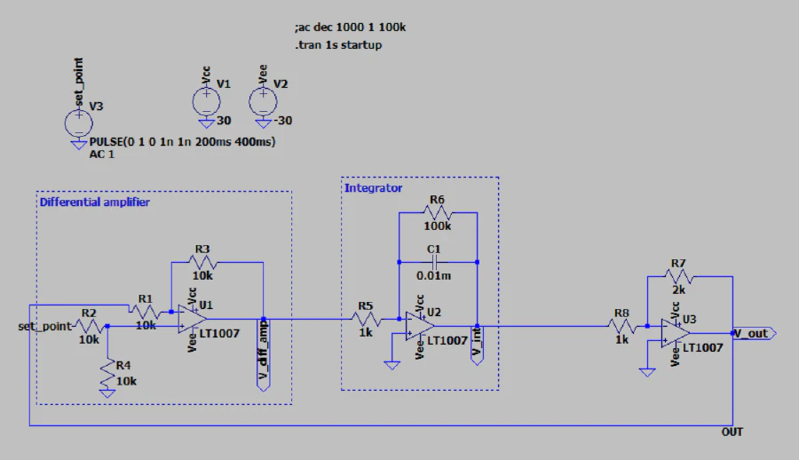
PI Controller with Square Wave Input
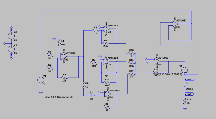
Circuit Diagram
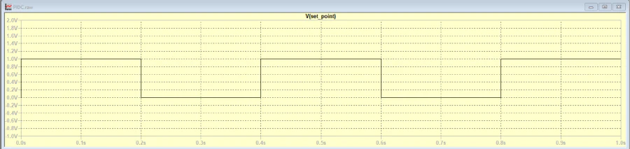
Setpoint
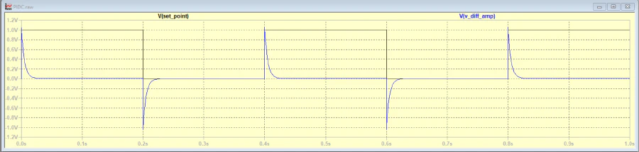
Output at Differential Amplifier
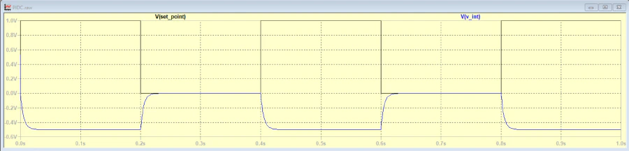
After Integral
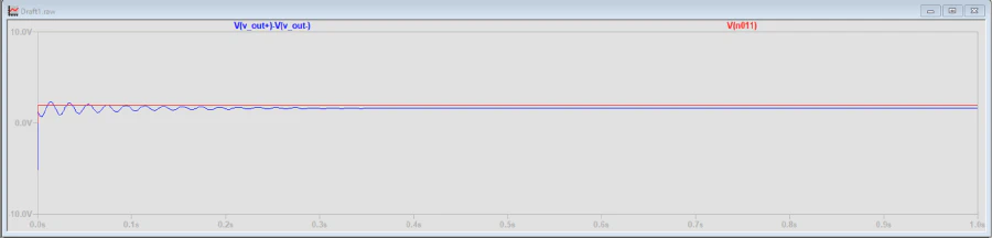
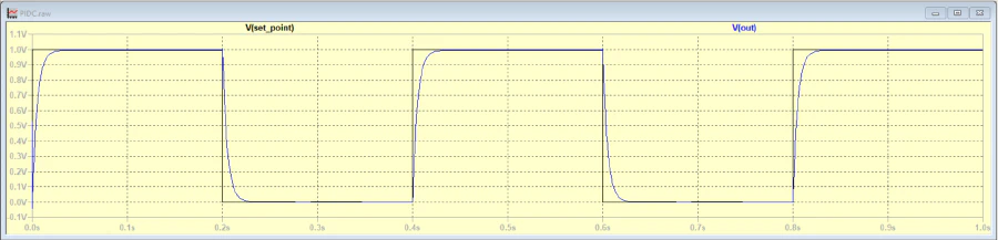
Final Output
PID Controller Transient Analysis
Circuit
Response