Jagadeesh Mummana | Portfolio

RU83C: Rubik’s Cube Solving Robot

Name	RU83C
Description	Rubik’s Cube-solving robot using Kociemba algorithm, featuring computer vision for state detection, mechanical design for cube manipulation, and electronics for execution.
Start	Ideation(July 2023), Implementation(Aug 2023)
Repository	RU83C🔗
Type	SOLO
Level	Beginner
Skills	Algorithms, Programming, Game Dev
Tools Used	Blender, Unity3D, Python, C#, VS Code, OpenCV, Fusion 360, ArduinoIDE
Current Status	Ongoing (Passive)
Progress	- Unity3D implementation is done. - Mechanical Design is started in Fusion 360 - CV part code is ready, color ranges yet to be tuned
Next Steps	- CV (Computer Vision): Responsible for recognizing the scrambled state of the cube via a camera. - Mechanical Design: Focused on the creation of the holder and gripping mechanisms to manipulate the cube. - Electronics: Controls and coordinates the robot’s movements based on the computed solution.

Overview

RU83C is a Rubik’s Cube-solving robot that leverages computer vision (CV), mechanical design, and electronics to solve a scrambled Rubik’s Cube using the Kociemba algorithm. The robot features a camera that captures the current state of the scrambled cube, processes the image using CV, and calculates the solution. A mechanical holder grips the cube securely, and the robot executes the necessary moves to solve it.

Features

Computer Vision: A camera-based system to detect the current state of the Rubik’s Cube, using image processing techniques to translate the visual input into a digital cube representation.

Mechanical Design: A custom-built holder with an efficient gripping system to securely hold and rotate the cube while executing the solution.

Kociemba Algorithm: The Kociemba algorithm is employed to calculate the optimal solution for the scrambled state.

Electronics: The system uses electronics to control the motors and mechanical components, translating the calculated moves into physical actions.

Structure

The project is divided into several key parts:

CV (Computer Vision): Responsible for recognizing the scrambled state of the cube via a camera.
Mechanical Design: Focused on the creation of the holder and gripping mechanisms to manipulate the cube.
Algorithm: Implementation of the Kociemba algorithm to calculate the solution to any scrambled state.
Electronics: Controls and coordinates the robot’s movements based on the computed solution.

Base Version

A base version of this project was previously developed in simulation, where users could manually or automatically scramble a virtual cube in Unity. The solution for the scrambled cube was calculated and displayed in the virtual environment. This was an intermediate step, and the current version represents the full hardware implementation of the Rubik’s Cube-solving robot.

BASE VERSION: here –implemented in simulation using Unity3D(C#)

BASE VERSION

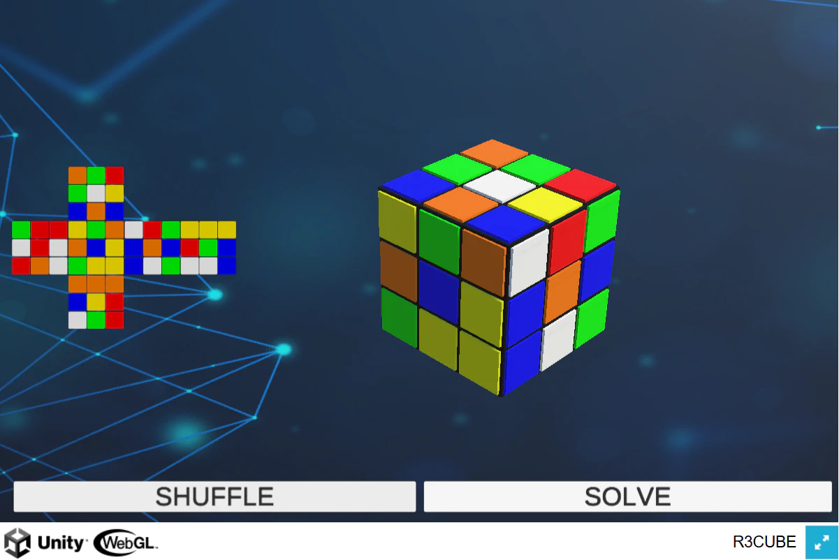
V-RU81K5CU83 - Virtual Rubik’s Cube Using Kociemba Solver

A virtual Rubik’s Cube implemented using the Kociemba algorithm for solving scrambled states. This project offers an interactive 3D simulation of a Rubik’s Cube that you can scramble, manipulate manually, and solve. The solution is computed using the Kociemba two-phase algorithm, widely known for its efficiency in solving Rubik’s cubes with minimal moves.

Deployment: This project is deployed using a WebGL server with Node.js alongside GitHub Pages for hosting the live demo.

INSPIRATION: @Megalomobile

Click here for the Live Demo | Vercel

Features

Interactive 3D Cube: Manipulate the cube by dragging and rotating different layers in 3D space.
Scramble & Solve: Automatically scramble the cube or solve any configuration using the Kociemba algorithm.
Unity/Blender Simulation: Visual simulations and demos showcasing the solution steps.

Demo Videos

Unity 3D Demo	Blender Solution Demo

Project Overview

This project leverages the pre-existing Kociemba two-phase algorithm for Rubik’s Cube solving, and our main contribution has been the seamless integration of this algorithm into a Unity-based simulation. The role of the solver is crucial, as it computes the solution when a scrambled cube is presented.

We designed the system to fetch cube states directly from the user interface, where users can scramble or manipulate the cube. Upon clicking the “Solve” button, the Kociemba algorithm works under the hood to generate an optimal solution, which is then passed to the Unity engine. The Unity environment simulates this solution visually, step by step, allowing users to see the cube’s transformation in real-time.

The Blender solution demo featured here is purely a visual mockup, simulating how the cube might appear when following a solved sequence. It serves as a demonstration for visual feedback but has no direct involvement in the solving process or algorithm implementation. This is an intermediate step showcasing the solution process and will be further integrated into Unity for enhanced user interaction.

Kociemba’s Algorithm for Solving a Rubik’s Cube

Kociemba’s Algorithm is a two-phase algorithm used to efficiently solve a 3×3 Rubik’s Cube in a minimal number of moves. It is an advanced method that improves upon simpler approaches, such as layer-by-layer (LBL) solving, by reducing the number of moves required to solve the cube.

Kociemba’s Algorithm is often used in optimal cube solvers, and it serves as the basis for algorithms like Herbert Kociemba’s Cube Explorer and the well-known Two-Phase Algorithm.

Overview of the Algorithm

The algorithm consists of two main phases:

Phase 1: Reducing the cube to a subset of solvable states known as the “G1 group”.
Phase 2: Solving the cube optimally from this subset.

By breaking the problem into these two phases, Kociemba’s Algorithm achieves solutions that typically require around 20 moves (or fewer), which is significantly shorter than beginner methods.

Mathematical Background

The algorithm relies on group theory, particularly the concept of cosets and group reductions. In simple terms, it works by reducing the number of legal states the cube can be in while maintaining solvability.

The Rubik’s Cube has a state space of 43,252,003,274,489,856,000 (43 quintillion) possible arrangements. Finding an optimal solution in this space is extremely complex, but by using the concept of group reduction, the problem is split into two more manageable parts.

PHASE 1: Reduction to G1 Group

In this phase, the cube is transformed into a restricted subset of states where:

All edge orientations are correct (edges are in the correct flipped orientation).
All corner orientations are correct.
The positioning of the U/D (Up/Down) face edges falls into a specific allowed pattern.

This phase does not solve the cube completely but simplifies it to a structured form that is easier to solve in the second phase.

Mathematical Properties of G1 Group

The group G1 is a subset of all possible cube states that satisfies the following conditions:

Edge Orientation is Solved: Each edge must be in its correct orientation.
Corner Orientation is Solved: Each corner must be in its correct orientation.
UD-Slice Edges Must Stay in the UD-Slice: The four edges belonging to the U (Up) and D (Down) face centers must remain within that slice.

The key insight is that reducing the cube to this state significantly reduces the number of possible positions, making the final solving phase much easier.

How This Phase Works

Kociemba’s algorithm uses a pruning table that precomputes the minimum number of moves required to reach the G1 state from any given configuration.
Using bidirectional search, the algorithm efficiently finds the shortest path to reach G1.
Typically, this phase takes at most 12 moves.

PHASE 2: Solving the Cube from G1

Once the cube is in the G1 subset, the next step is to solve it completely while maintaining the constraints of G1.

Mathematical Properties of Phase 2

In this phase, we solve the cube while ensuring:

The E-Slice (Middle Layer Edges) is Correct: The four middle layer edges must be correctly positioned.
Corner Permutation is Correct: The corners must be arranged correctly.
Edge Permutation is Correct: All edges must be positioned correctly.

At this point, the cube is already simplified, so a brute-force or optimized search (using a pruning table) is performed to find the shortest solution sequence.

This phase usually takes around 10 moves in most cases.
Since the cube is already in a reduced state, only a limited number of moves are needed to reach the solved state.

Key Techniques Used in Kociemba’s Algorithm

Pruning Tables

The algorithm precomputes lookup tables that store the shortest paths for solving different cube states.
These tables help the algorithm efficiently determine the best next move without unnecessary computations.

Heuristic Search

Kociemba’s Algorithm uses A search* (or similar algorithms) to minimize the number of moves required to reach a solved state.
It evaluates different move sequences and picks the shortest one.

Group Theory-Based Reduction

The algorithm does not directly solve the cube but instead reduces it step by step to smaller solvable subsets.
By using cosets and subgroups, the problem is broken down into manageable parts.

Move Pruning & Bidirectional Search

The algorithm avoids unnecessary moves by pruning branches that lead to longer solutions.
It uses bidirectional search (searching both forward and backward) to quickly find the optimal solution.

Why is Kociemba’s Algorithm Efficient?

It significantly reduces the search space: Instead of searching through 43 quintillion possible states, it first reduces the cube to G1, making the search much easier. It finds near-optimal solutions: While not always the absolute shortest solution, Kociemba’s Algorithm typically finds solutions within 20 moves, close to the God’s Number (20 moves). It is practical for human and computer solvers: Many advanced cube solvers and speedcubing programs use this approach for efficient solving.

Comparison to Other Solving Methods

Algorithm	Average Move Count	Approach
Layer-by-Layer (Beginner Method)	100+ moves	Step-by-step solving
CFOP (Fridrich Method)	50-60 moves	Speedcubing method
Kociemba’s Algorithm	~20 moves	Two-phase optimal solving
Thistlethwaite’s Algorithm	40-50 moves	Four-phase group theory approach
God’s Algorithm	20 moves (optimal)	Brute-force minimum solution

Kociemba’s Algorithm is not always optimal, but it is extremely efficient and can be computed very quickly compared to brute-force approaches.

Applications of Kociemba’s Algorithm

Speedcubing: Used in optimal cube-solving software.
Computer Solvers: Implemented in AI-based solvers and robotic Rubik’s Cube solvers.
Mathematical Research: Used to study group theory and combinatorial optimization.
God’s Number Research: Helps find efficient solutions near the 20-move optimal bound.

Controls

Right Click + Drag: Rotate the entire cube in 3D space.
Left Click + Drag on Layers: Rotate specific layers of the Rubik’s Cube.

Buttons

SCRAMBLE: Randomly scrambles the Rubik’s Cube.
SOLVE: Solves the scrambled cube using the Kociemba solver. (Note: Initial solve may take some time to compute.)

Layout

Installation & Setup

To run the project locally, follow these steps:

Clone the repository:

git clone https://github.com/Mummanajagadeesh/v-rubiks-cube.git
cd v-rubiks-cube

Open the project in your preferred IDE or deploy it on a web hosting service.
To modify or extend the project, ensure you have:
- A working knowledge of 3D engines such as Unity or Blender.
- Familiarity with the Kociemba algorithm and basic Rubik’s Cube concepts.

How the Solver Works

This project uses the Kociemba two-phase algorithm, which is an optimized approach for solving the Rubik’s Cube in under 20 moves. The first phase reduces the problem to a manageable subset of configurations, and the second phase finds an optimal solution from that subset.

Performance Notes

The first time you run the solver, it may take longer due to the initial calculation of move tables.
Subsequent solves will be faster as the tables are cached.

Future Goals

We have exciting plans for the future of this project:

Hardware Integration: The next step is to bring this solution into the physical world. Using computer vision (CV) techniques, we aim to read the Rubik’s Cube faces via a camera and translate the detected state into a solvable format.
3D Design: We are currently working on the 3D design of the hardware, which is under construction. This will involve a mechanism where gripper-like structures hold and manipulate the cube for solving.
Optimization: Another goal is to reduce the time required for solving, making the process as fast and efficient as possible.
Physical Cube Solving: Ultimately, the project will be able to solve a real Rubik’s Cube using robotic structures that simulate the virtual environment.

We are open to contributions from anyone interested in participating in this exciting journey. If you’d like to help us push the project forward, feel free to reach out!

Enjoy solving the cube! 🎲