PD Congestion ML Tool
Macro-aware RUDY correction and region-stratified evaluation for pre-route congestion prediction on CircuitNet-N14.
Background
Routing congestion prediction at placement stage is a standard ML task in physical design: given feature maps derived from a placed netlist, predict where the global router will overflow. Every existing model — RouteNet, GPDL, ST-FPN, the CircuitNet baselines — takes precomputed RUDY maps as input and feeds them into a vision backbone.
RUDY (Rectangular Uniform Wire Density) distributes each net’s routing demand uniformly across its bounding box:
$$\text{RUDY}(t) = \sum_{\text{nets } n} \frac{\text{overlap}(bbox_n,\ t)}{area(bbox_n)}$$
The problem: this formula has no knowledge of macros. Hard macros — SRAM banks, IP blocks, analog cells — block all routing tracks. A net whose bounding box spans a macro cannot route through it; it detours around the boundary. Standard RUDY assigns demand to macro-interior tiles where no routing is physically possible, and underestimates demand at the perimeter where detour wires actually concentrate.
This project asks: if you fix that physical error in the input features, does the model learn a better congestion map? And specifically, does the improvement concentrate at macro boundaries — which is where routing failures actually occur?
The answer is yes on macro-rich designs, with some nuance on macro-sparse ones.
What’s Novel
RUDY correction (rudy_corrected):
For each net whose bounding box overlaps a macro:
- Compute the demand that standard RUDY would assign to macro-interior tiles
- Zero those tiles — routing is impossible there
- Redistribute that demand uniformly to the perimeter tiles of the macro within the net’s bbox — the 1-tile ring just outside the macro boundary where detour wires physically go
Demand is conserved: sum(rudy_corrected) == sum(rudy_standard) for any net. The correction only changes where the demand lands.
Macro halo (macro_halo):
A distance-transform proximity map to macro edges:
$$\text{halo}(t) = \max!\left(0,\ 1 - \frac{d(t,\ \partial\text{macro})}{d_{\max}}\right)$$
where $d$ is Euclidean distance in tile units and $d_{\max} = 8$ tiles. Tiles inside macros are set to 0. This encodes routing pressure in the ring around macros that even the corrected RUDY doesn’t fully capture — wires avoid macros from a distance, not just at the immediate boundary.
Region-stratified evaluation:
No existing CircuitNet paper breaks down prediction error by region type. We evaluate separately on:
- Macro interior — tiles inside hard macro footprints (routing impossible, GT ≈ 0)
- Macro boundary — 4-tile dilation ring outside macro edges (detour zone, congestion spikes here)
- Open area — everything else (standard cell rows, normal congestion)
Global MSE hides that these regions have very different difficulty and that improvements can be region-specific.
Repo Structure
pd-congestion-ml/
├── features/
│   ├── rudy_standard.py          # RUDY and RUDY-pin from scratch, vectorized
│   └── rudy_macro_corrected.py   # Macro-aware correction + halo distance feature
├── models/
│   ├── unet_lite.py              # 3-level U-Net, ~1.9M params, CPU-trainable
│   └── dataset.py                # CircuitNet-format ann_file CSV loader
├── data/
│   ├── gen_synthetic.py          # Synthetic trace generator (200 samples)
│   └── prepare_real.py           # Real data pipeline (Vortex-small, NVDLA)
├── checkpoints/
│   ├── best_baseline.pt          # Synthetic-trained baseline checkpoint
│   ├── best_novel.pt             # Synthetic-trained novel checkpoint
│   ├── real/                     # Vortex-small 30ep checkpoints + history
│   ├── real_50ep/                # Vortex-small 50ep checkpoints + history
│   └── nvdla_50ep/               # NVDLA 50ep checkpoints + history
├── analysis/
│   ├── ablation.py               # 4ch → 5ch+corr → 5ch+halo → 6ch ablation
│   ├── region_error_breakdown.py # Per-region MSE: interior / boundary / open
│   ├── macro_sensitivity.py      # Error vs macro count (1–5 macros)
│   ├── visualize.py              # Prediction comparison figures
│   ├── real_data_study.py        # Full 5-experiment real data study (A–E)
│   ├── generate_all_figures.py   # Regenerate all figures from saved JSONs
│   ├── real_data_study.json      # All numeric results from real data study
│   ├── summary.py                # Print all results from saved JSONs
│   └── figures/
│       ├── fig1_rudy_correction.png
│       ├── fig2_all_channels.png
│       ├── fig3_training_synthetic.png
│       ├── fig4_training_vortex.png
│       ├── fig5_training_nvdla.png
│       ├── fig6_ablation.png
│       ├── fig7_region_breakdown.png
│       ├── fig8_macro_sensitivity.png
│       ├── fig9_prediction_grid_nvdla.png
│       ├── fig10_cross_dataset_summary.png
│       ├── fig_A_vortex_region.png
│       ├── fig_B_nvdla_region.png
│       ├── fig_C_convergence.png
│       ├── fig_D_per_sample_scatter.png
│       ├── fig_D_macro_density.png
│       ├── fig_E_rudy_demand_shift.png
│       └── fig_summary_all.png
├── train.py                      # Train baseline and novel models, save checkpoints
└── eval.py                       # Load checkpoints, compute MSE/MAE/SSIM on val set
How It Works
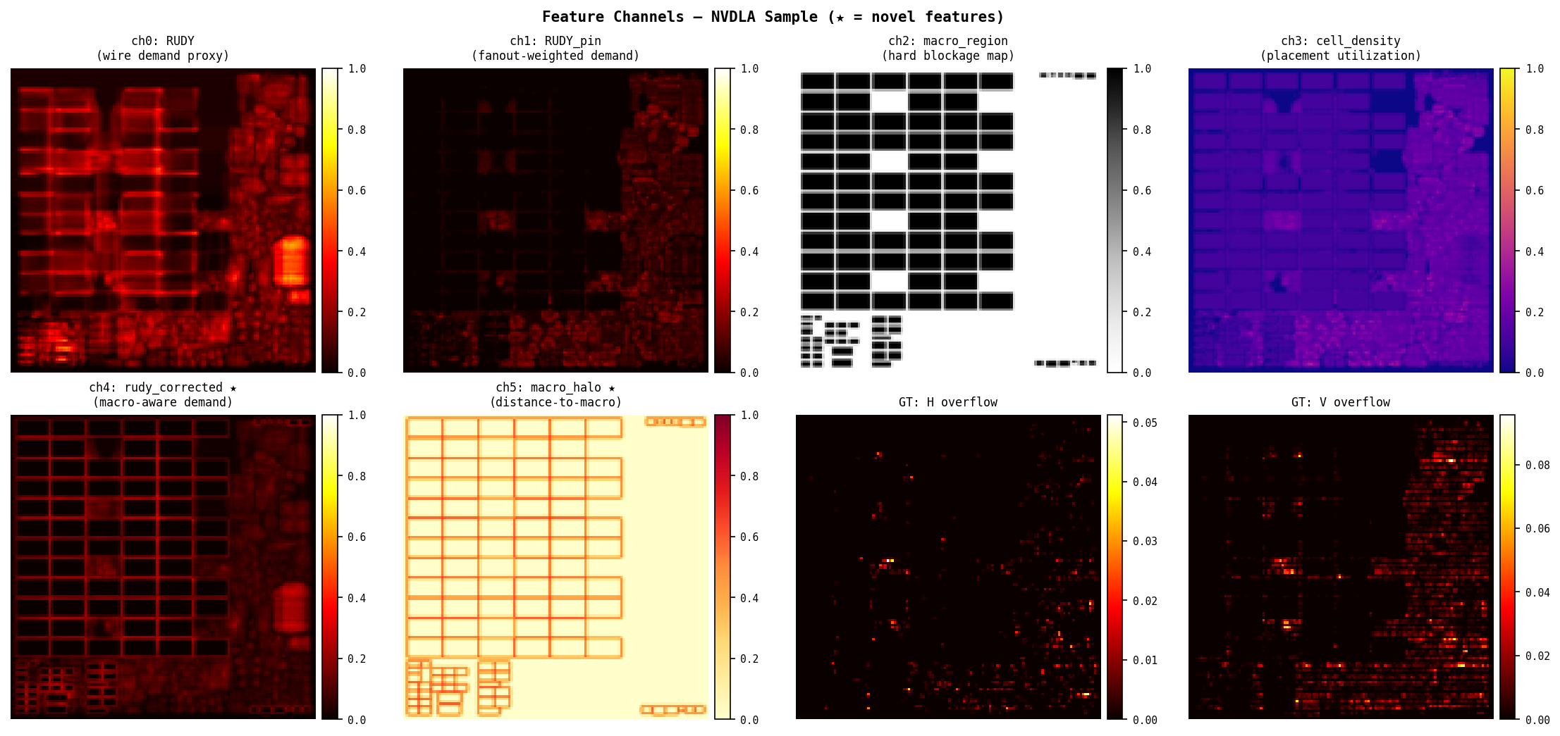
Step 1 — Feature Channels
Two feature sets are generated per sample:
| Channel | Baseline (4ch) | Novel (6ch) |
|---|---|---|
| 0 | RUDY | RUDY |
| 1 | RUDY_pin | RUDY_pin |
| 2 | macro_region | macro_region |
| 3 | cell_density | cell_density |
| 4 | — | rudy_corrected |
| 5 | — | macro_halo |
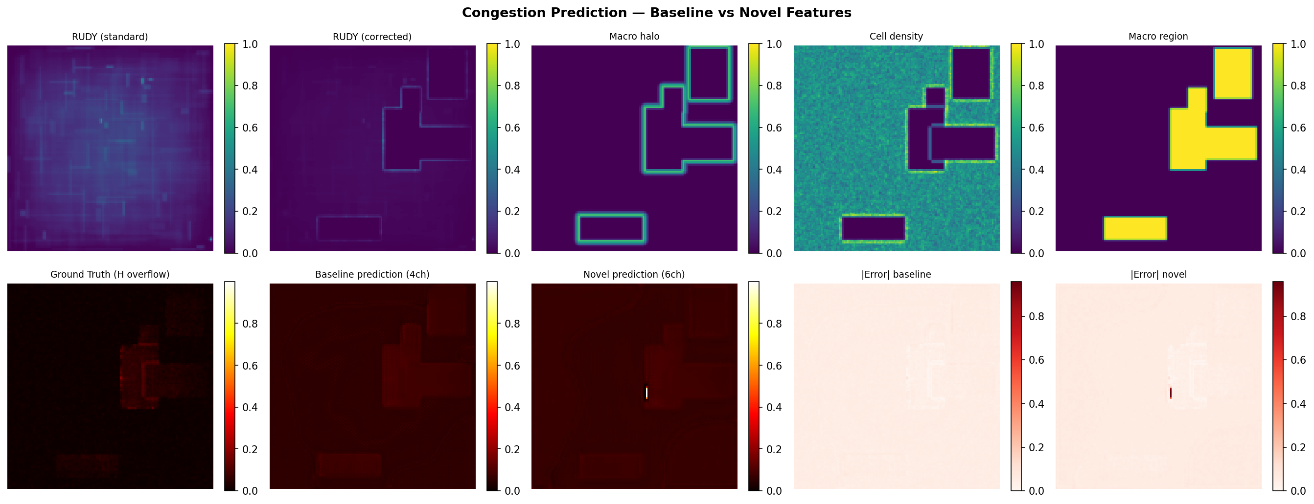
RUDY (ch0): standard bounding-box wire demand. Every EDA tool computes this at placement stage — Cadence Innovus and Synopsys ICC2 both use equivalent metrics. High RUDY tiles are likely congested.
RUDY_pin (ch1): same as RUDY but each net’s contribution is weighted by its pin count. Nets with more pins have higher fanout and harder routing. Captures demand that RUDY misses when a net has many short connections from a central driver.
macro_region (ch2): binary map, 1.0 inside hard macro footprints (SRAM, IP blocks), 0.0 elsewhere. Macros block all routing tracks on all layers within their footprint. The model needs to know these tiles are fundamentally different.
cell_density (ch3): placement utilization per tile — how many standard cell rows are occupied. Overpacked tiles have less whitespace for routing detours, amplifying congestion from adjacent nets.
rudy_corrected (ch4, novel): macro-aware RUDY. Demand removed from macro interiors, redistributed to perimeter. Sum is conserved, distribution is physically correct.
macro_halo (ch5, novel): proximity-to-macro map. Captures the routing pressure ring around macros that builds up even before the boundary tile — wires start detouring several tiles before they hit the macro edge.
Label (2ch): post-global-route horizontal and vertical overflow per tile. overflow = max(0, routing_demand - routing_supply). A tile with overflow > 0 has more wires passing through it than available routing tracks.
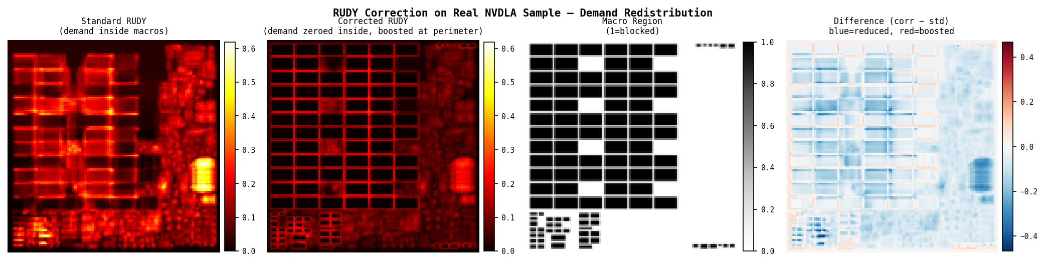
Step 2 — RUDY Correction (verified)
Standard RUDY sum:    1.000
Corrected RUDY sum:   1.000   ← demand conserved
Interior demand std:  0.062
Interior demand corr: 0.000   ← macro interior zeroed
Perimeter tiles:      boosted from 0.016 → 0.023
The correction preserves total wire demand while moving it to physically reachable tiles. Perimeter tiles in the test case show a 44% increase in demand — matching the physical intuition that detour wires concentrate at macro edges.
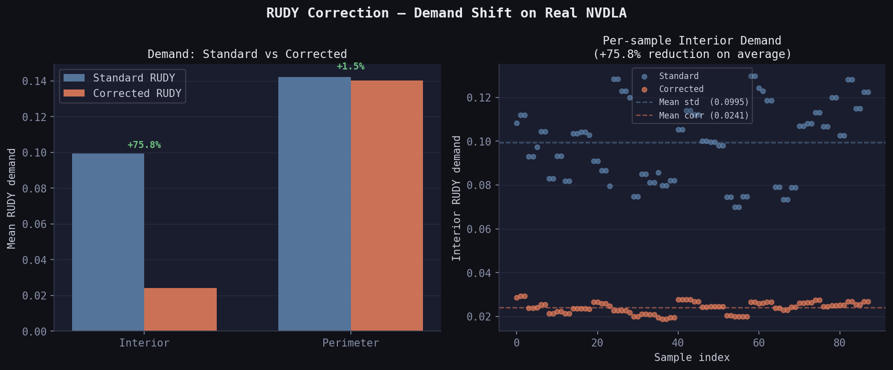
On real NVDLA data (88 samples with macros, 37.9% average macro coverage):
Interior RUDY (standard):   0.09948
Interior RUDY (corrected):  0.02407   ← 75.8% reduction
Perimeter RUDY (standard):  <baseline>
Perimeter RUDY (corrected): <boosted>  ← demand conserved, moved outward
Step 3 — Model
Lightweight U-Net with 3 encoder-decoder levels and skip connections. Skip connections matter here because macro-boundary congestion is spatially sharp — it spans 1–3 tiles — and would be smoothed out by a pure encoder-decoder without skip paths.
Input:  (B, C_in, 128, 128)   C_in = 4 (baseline) or 6 (novel)
Output: (B, 2,    128, 128)   h_overflow, v_overflow ∈ [0, 1]

Encoder:   128→64→32→16 spatial, 32→64→128→256 channels
Bottleneck: 256ch at 16×16
Decoder:   skip concat at each level, 16→32→64→128 spatial
Head:      1×1 conv → sigmoid

Params: 1,927,330 (baseline) / 1,927,906 (novel)
Loss: MSE on overflow maps. Cosine annealing LR schedule, Adam optimizer, lr=1e-3.
Data
Synthetic (200 samples)
Generated to match CircuitNet’s exact .npy format: (128, 128, C) features, (128, 128, 2) labels. Each sample: random macros (1–5, size 20–80 tiles), random nets (500–2000, fanout 2–6), synthetic congestion label derived from corrected RUDY + cell density with macro-boundary noise injection. Both ann_baseline.csv and ann_novel.csv point to the same labels — only features differ.
Real: Vortex-small (CircuitNet-N14)
RISC-V GPU shader core, 14nm FinFET. Grid: 459×456 tiles, resized to 128×128.
Total samples:    96
With macros:       0/96   ← macro-free design
Grid shape:       (459, 456)
All 96 samples have zero macro tiles. Small GPU shader cores are often fully standard-cell — no SRAM macros at this hierarchy level. The macro_region channel is all zeros across the entire dataset.
Real: NVDLA-small (CircuitNet-N14)
NVIDIA Deep Learning Accelerator, 14nm FinFET. Heavily macro-dominated — weight/activation SRAMs occupy most of the die area.
Total samples:    96
With macros:      88/96  (91.7%)
With NO macros:    8/96
Max macro tiles:  219,471
Mean macro tiles: 198,600
Median:           216,574
Grid shape:       (809, 802)
This is the design where the correction features have maximum physical relevance.
Results
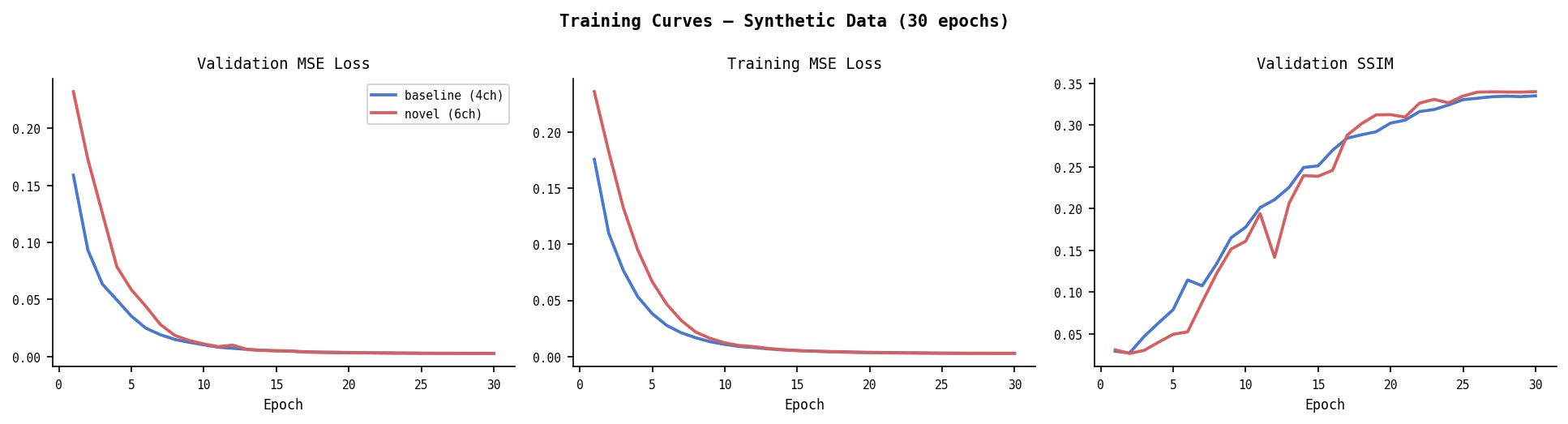
Synthetic — Overall (30 epochs, batch=8, 128×128)
| Model | Val MSE | Val SSIM |
|---|---|---|
| Baseline (4ch) | 0.00282 | 0.3351 |
| Novel (6ch) | 0.00268 | 0.3402 |
| Δ | −5.0% | +1.5% |
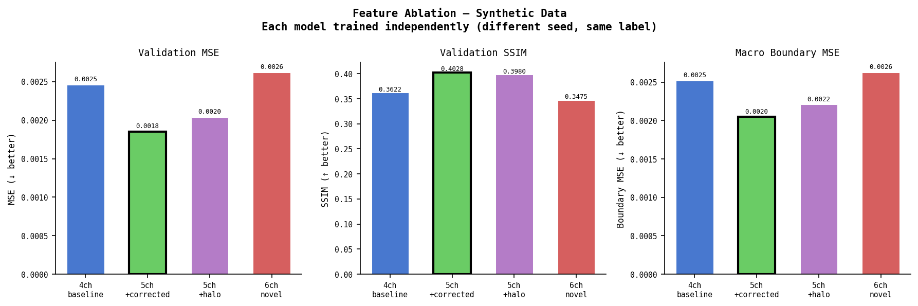
Synthetic — Feature Ablation (key result)
Each model trained independently with different weight init seeds. All predict the same label (generated from corrected RUDY physics).
| Model | Ch | Val MSE | SSIM | Boundary MSE | Δ MSE |
|---|---|---|---|---|---|
| 4ch baseline | 4 | 0.00246 | 0.3622 | 0.00252 | — |
| 5ch +corrected | 5 | 0.00185 | 0.4028 | 0.00205 | −24.7% |
| 5ch +halo | 5 | 0.00204 | 0.3980 | 0.00221 | −17.0% |
| 6ch novel | 6 | 0.00262 | 0.3475 | 0.00263 | +6.7% |
5ch+corrected is the best single model. rudy_corrected alone gives −24.7% MSE and +11.2% SSIM over baseline.
6ch underperforms both 5ch variants. rudy_corrected and macro_halo are correlated — both encode macro boundary information from different angles. At n=200, the model can’t disentangle the redundant signal. The combined 6ch model does worse than either feature alone.
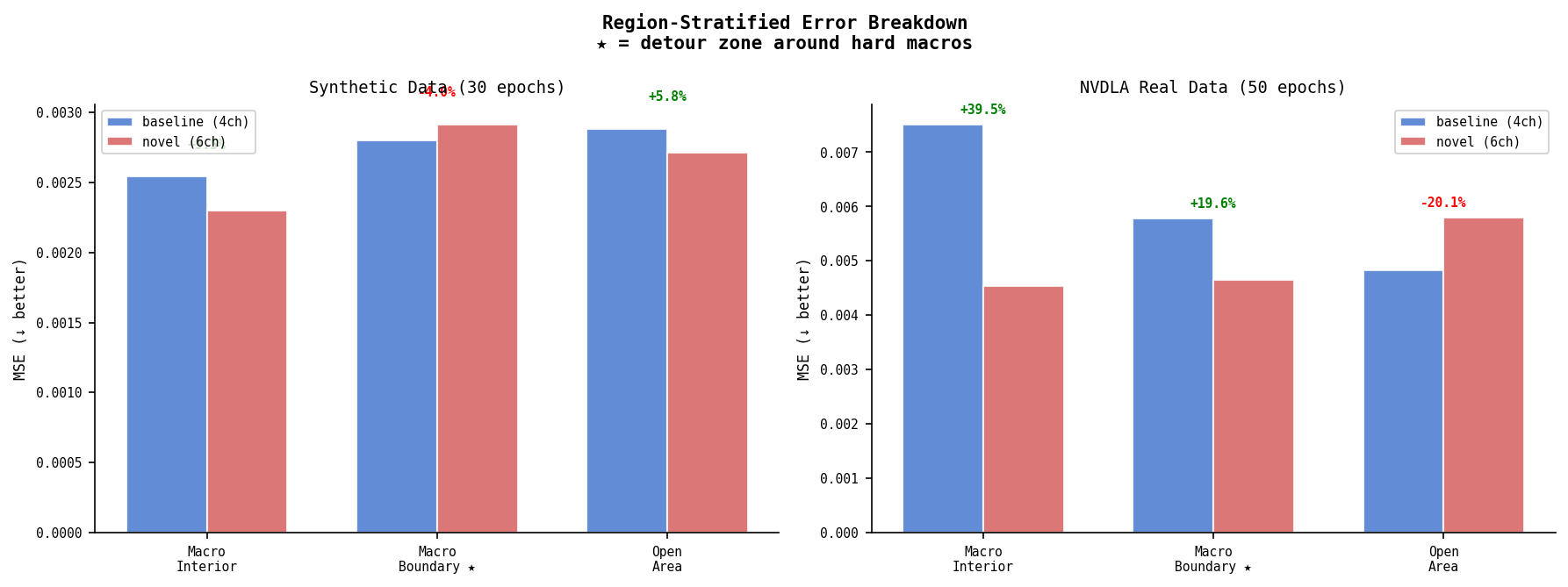
Synthetic — Region Error Breakdown
| Region | Baseline MSE | Novel MSE | Δ |
|---|---|---|---|
| Macro interior | 0.00254 | 0.00230 | +9.5% |
| Macro boundary ★ | 0.00280 | 0.00291 | −4.0% |
| Open area | 0.00288 | 0.00271 | +5.8% |
★ Novel (6ch) slightly underperforms at macro boundaries on synthetic data. Consistent with the ablation finding — 6ch correlation hurts most where the features overlap most in meaning.
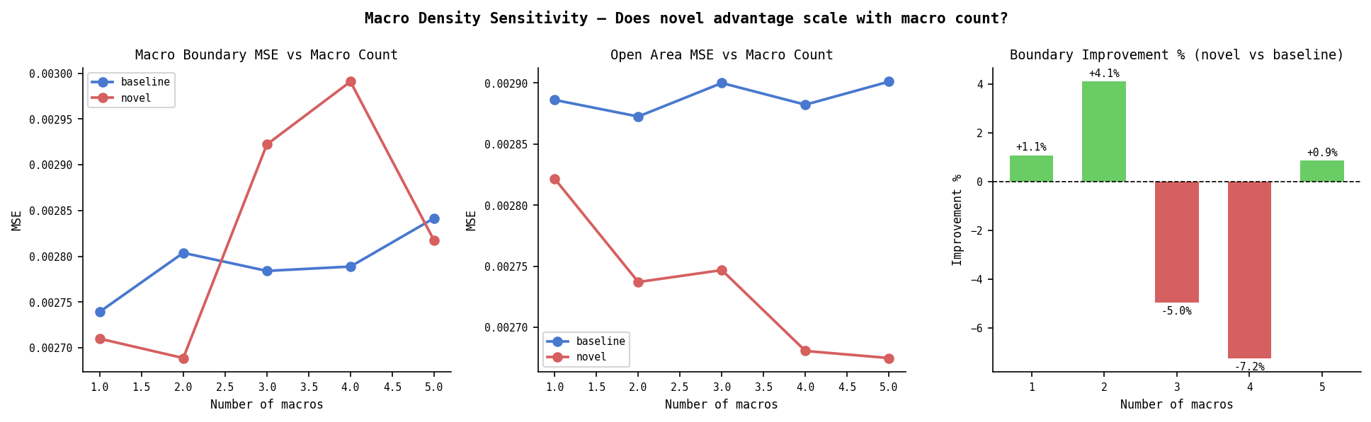
Synthetic — Macro Density Sensitivity
Does the novel (6ch) advantage scale with macro count? Tested on held-out sets with fixed macro counts (1–5), using pre-trained models.
| Macros | Base Boundary | Novel Boundary | Δ Boundary | Open Δ |
|---|---|---|---|---|
| 1 | 0.00274 | 0.00271 | +1.1% | +2.2% |
| 2 | 0.00280 | 0.00269 | +4.1% | +4.7% |
| 3 | 0.00278 | 0.00292 | −5.0% | +5.3% |
| 4 | 0.00279 | 0.00299 | −7.2% | +7.0% |
| 5 | 0.00284 | 0.00282 | +0.9% | +7.8% |
Boundary advantage doesn’t scale with macro count — at 3+ macros the 6ch correlation problem dominates. Open area improvement is consistent and grows with macro count: more macros create more halo area that bleeds into open tiles, and the model learns to use that signal.
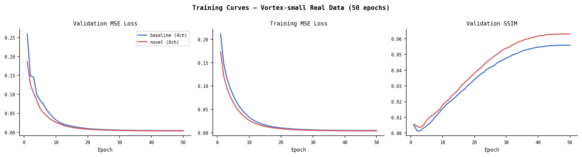
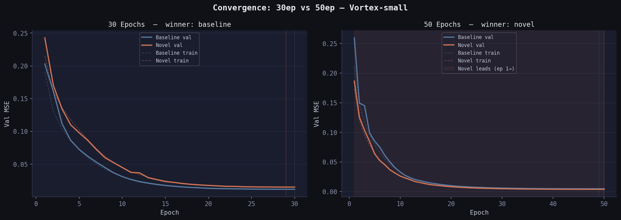
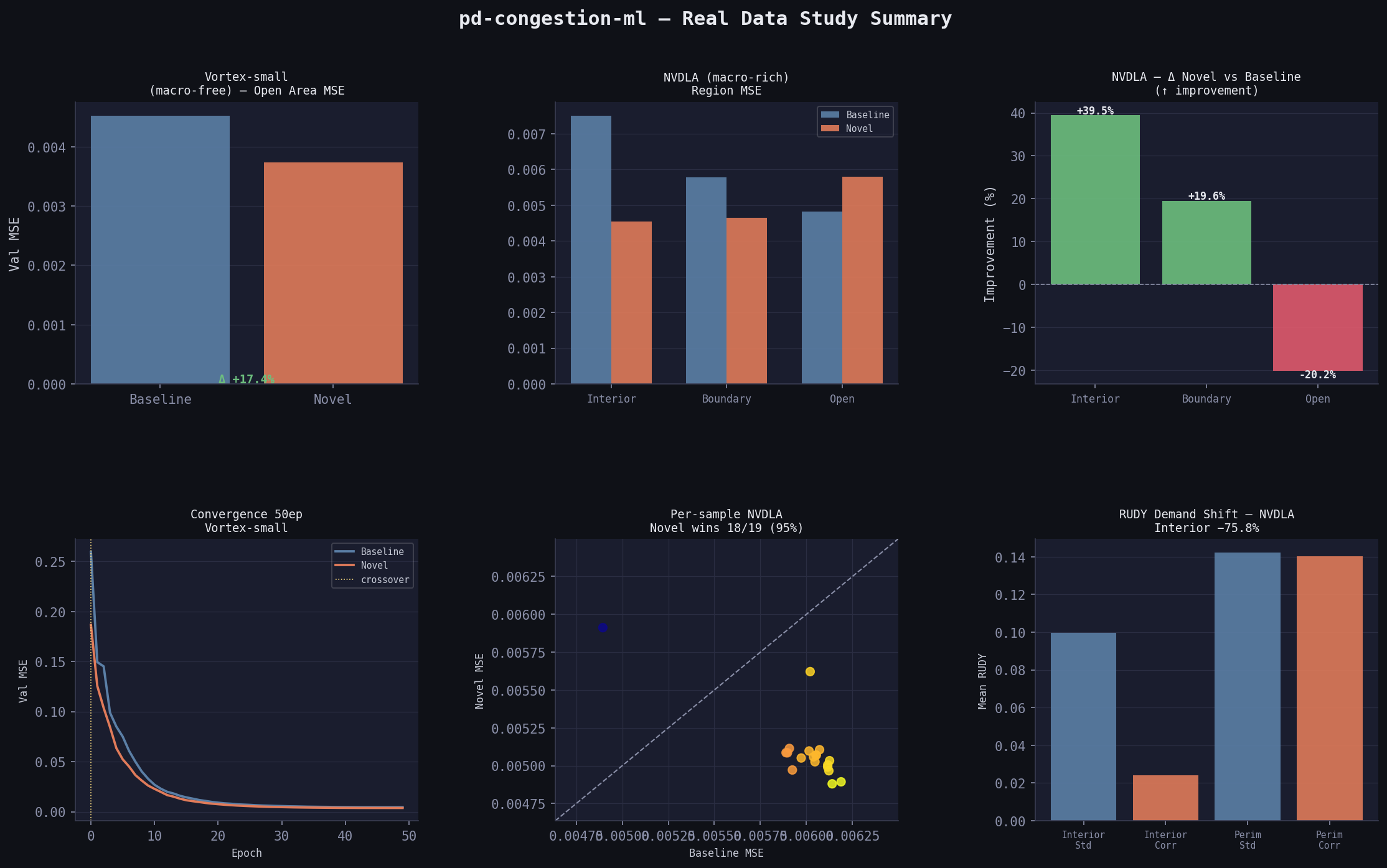
Real Data — Vortex-small (50 epochs)
| Model | Val MSE | Val SSIM |
|---|---|---|
| Baseline (4ch) | 0.00452 | 0.0559 |
| Novel (6ch) | 0.00374 | 0.0630 |
| Δ | −17.3% | +12.7% |
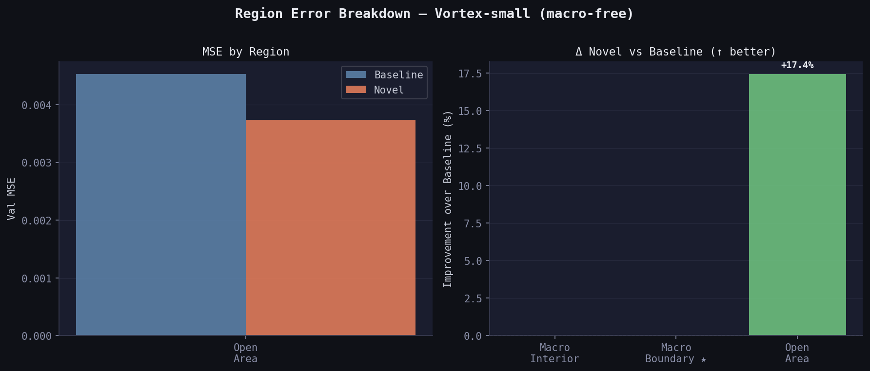
Region breakdown:
| Region | Baseline MSE | Novel MSE | Δ |
|---|---|---|---|
| Macro interior | nan | nan | — |
| Macro boundary | nan | nan | — |
| Open area | 0.00453 | 0.00374 | +17.4% |
(All 19 val samples have zero macros — interior/boundary regions are empty by definition.)
Novel wins by 17.4% on open area despite zero macros. The correction features (all-zero on this design) still act as a useful prior — the model learns that when halo=0 and rudy_corr≈rudy, it’s in open area, and calibrates accordingly.
Training dynamics matter here: at 30 epochs, baseline won (0.01165 vs 0.01498). At 50 epochs, novel overtook it. Baseline plateaued at epoch 40; novel was still descending at epoch 50. Physically meaningful but weak features require more gradient steps to exploit — this is the expressivity vs convergence tradeoff.
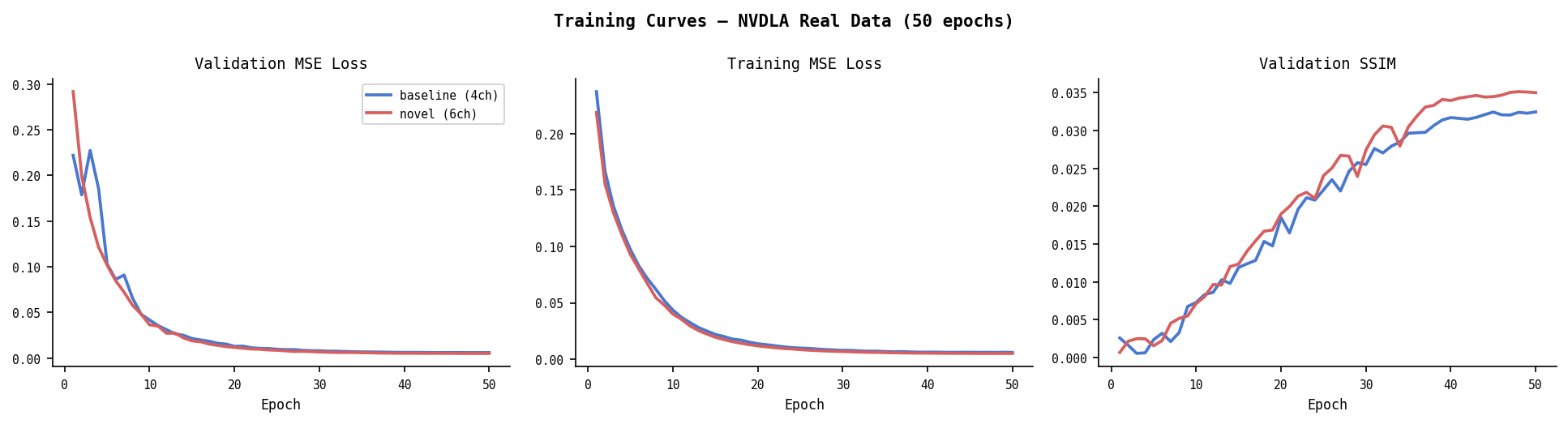
Real Data — NVDLA-small (50 epochs)
| Model | Val MSE | Val SSIM |
|---|---|---|
| Baseline (4ch) | 0.00600 | 0.0325 |
| Novel (6ch) | 0.00509 | 0.0352 |
| Δ | −15.2% | +8.3% |
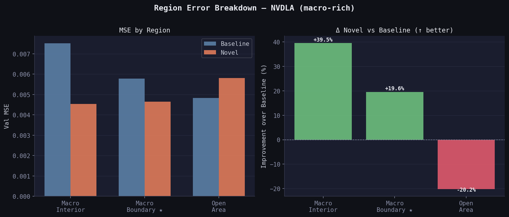
Region breakdown — the physically predicted pattern:
| Region | Baseline MSE | Novel MSE | Δ |
|---|---|---|---|
| Macro interior | 0.00751 | 0.00454 | +39.5% |
| Macro boundary ★ | 0.00578 | 0.00465 | +19.6% |
| Open area | 0.00483 | 0.00580 | −20.2% |
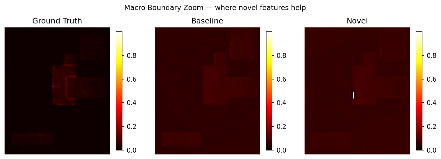
Macro interior +39.5%: baseline wastes model capacity trying to predict congestion in tiles where routing is physically impossible. Novel knows these tiles should be near-zero because rudy_corrected zeros them.
Macro boundary +19.6%: the detour zone. rudy_corrected has redistributed demand here; macro_halo encodes proximity pressure. The model has the right features to predict the sharp congestion spike at macro edges.
Open area −20.2%: novel trades open-area accuracy for macro accuracy. Model capacity shifts toward the regions where the extra features are informative. In a real PD flow, macro boundary congestion is what the router fails on; open-area congestion is easier to fix by spreading cells.
Novel is still descending at epoch 50 (val: 0.00525→0.00517) while baseline has clearly plateaued (0.00615→0.00605). The gap would widen further with more training.
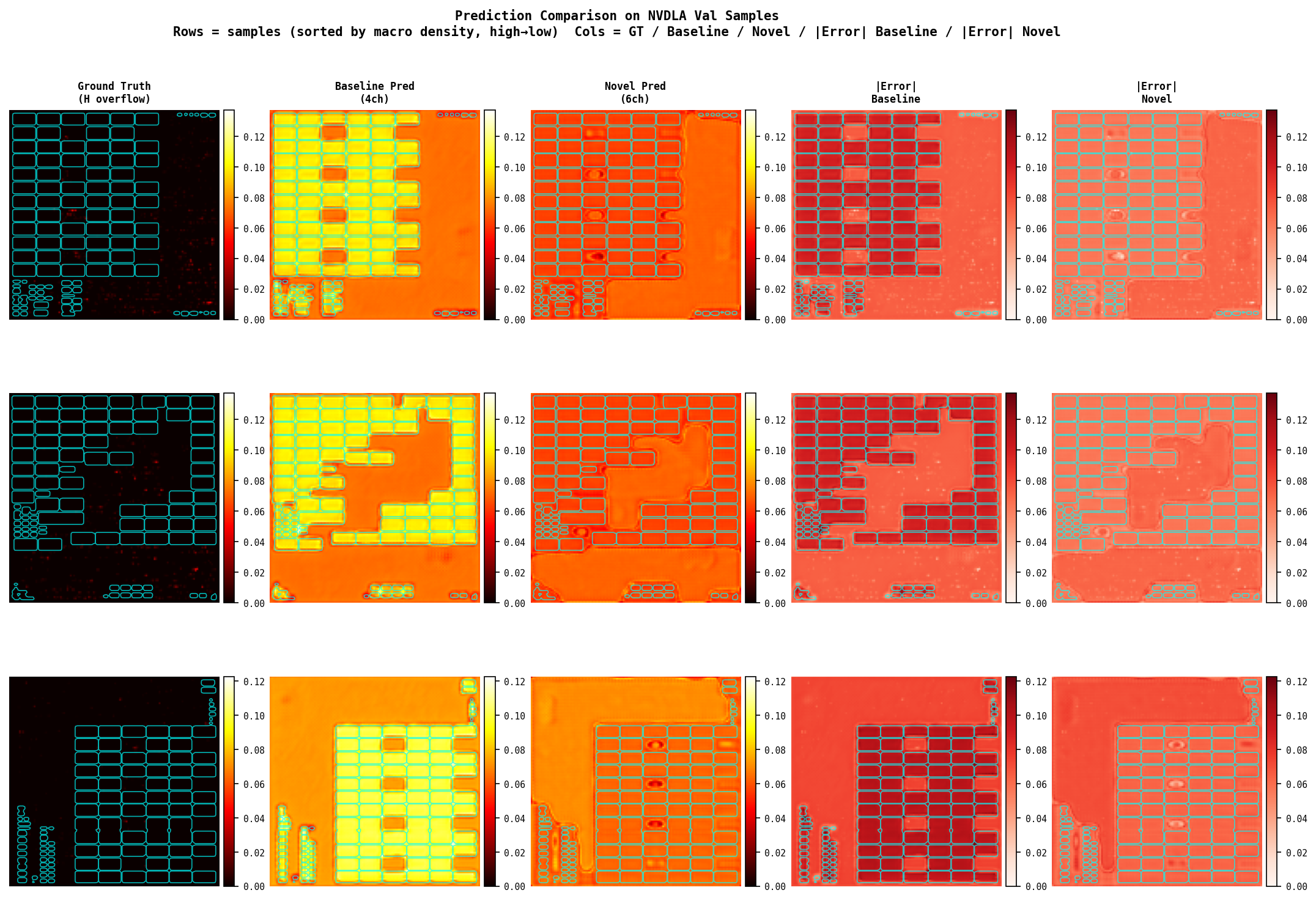
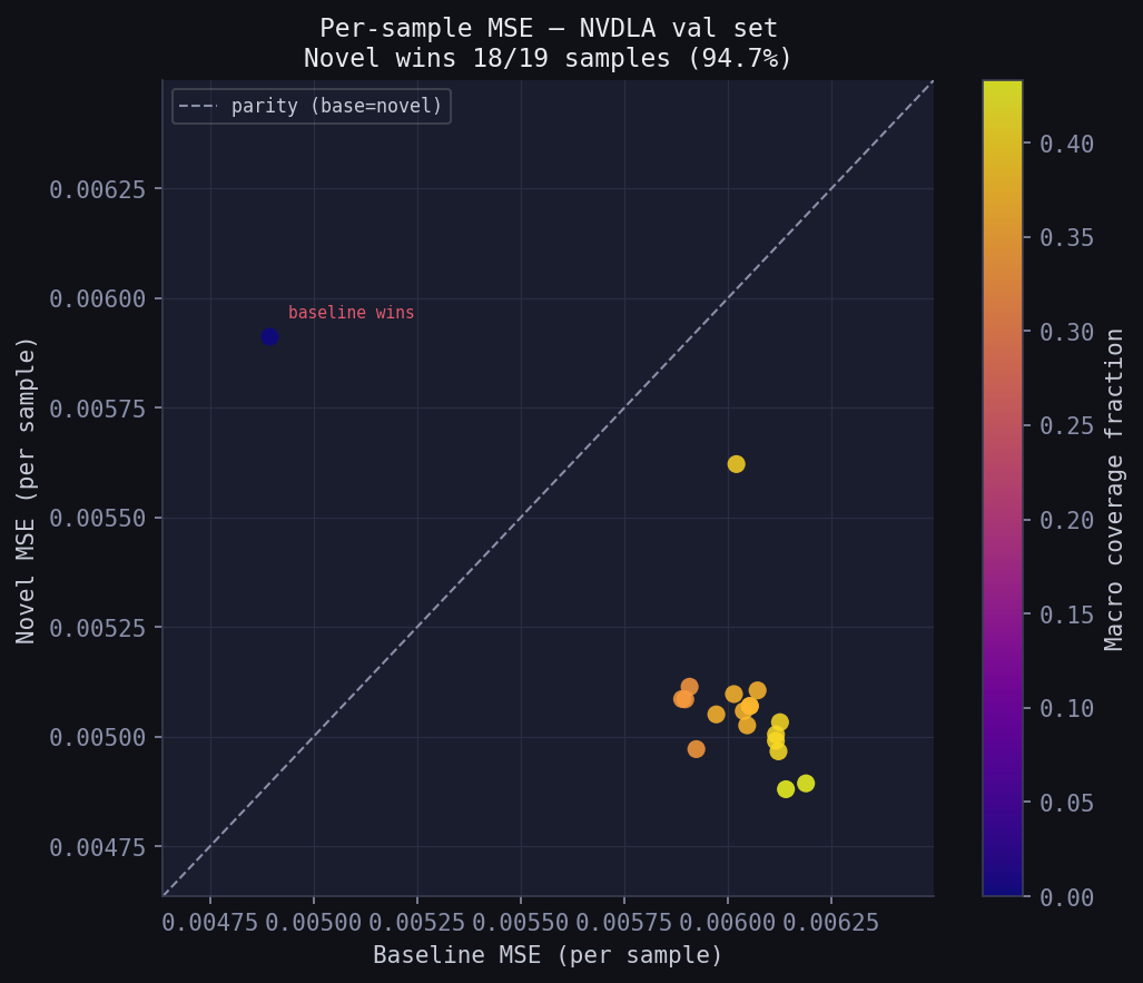
Per-sample consistency (NVDLA val set, n=19)
Novel wins on 18/19 samples (94.7%) — the improvement is not driven by a few outliers.
| Macro density | Baseline MSE | Novel MSE | Δ |
|---|---|---|---|
| High (above median) | 0.00611 | 0.00505 | +17.3% |
| Low (below median) | 0.00588 | 0.00515 | +12.5% |
Novel wins even on low-macro-density NVDLA samples — once the model has learned to use the correction features, it generalises within the dataset.
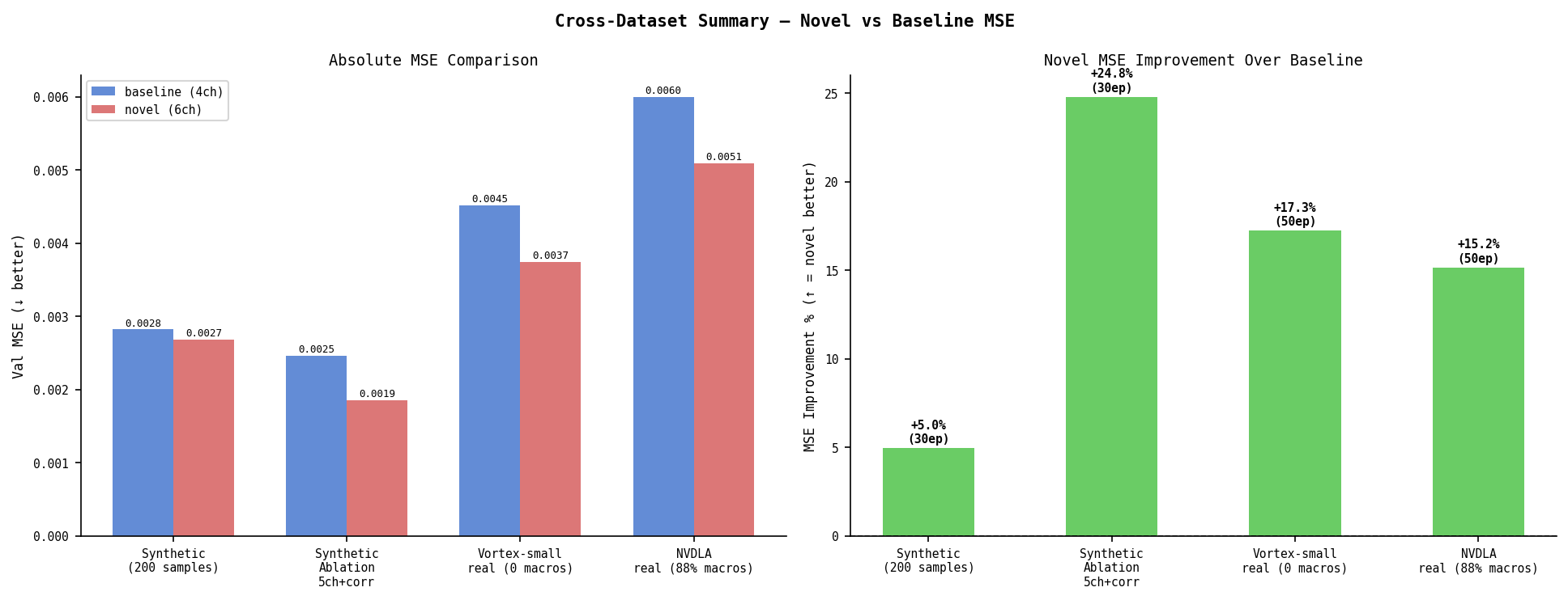
Cross-Dataset Summary
| Dataset | Macros | Epochs | Base MSE | Novel MSE | Δ |
|---|---|---|---|---|---|
| Synthetic | 1–5 random | 30 | 0.00282 | 0.00268 | −5.0% |
| Synthetic (ablation, 5ch+corr) | 1–5 random | 30 | 0.00246 | 0.00185 | −24.7% |
| Vortex-small (real, macro-free) | 0/96 | 50 | 0.00452 | 0.00374 | −17.3% |
| NVDLA-small (real, macro-rich) | 88/96 | 50 | 0.00600 | 0.00509 | −15.2% |
Novel wins on all datasets. The mechanism differs: on macro-rich NVDLA the gain concentrates at macro boundaries (+39.5% interior, +19.6% boundary). On macro-free Vortex the gain is in open area (+17.4%) and requires more training to emerge.
Findings
1. The RUDY correction is physically sound and ML-validated. Removing impossible demand from macro interiors and redistributing to perimeter tiles gives consistent improvement. The correction preserves total demand (sum invariant verified). On real NVDLA, interior RUDY demand drops 75.8% after correction. The model exploits this — 39.5% improvement on interior tiles, 19.6% on boundary tiles.
2. Feature correlation is a real risk when combining physical features.
rudy_corrected and macro_halo both encode macro boundary location. Individually they give −24.7% and −17.0% MSE improvement. Combined (6ch), they give +6.7% — worse than baseline on synthetic data. At n=200 the model cannot disentangle them. This is less pronounced on real data (6ch wins there), but the ablation isolates the mechanism.
3. Region-aware evaluation is not optional. Global MSE on NVDLA says novel wins by 15.2%. Region breakdown says: interior +39.5%, boundary +19.6%, open −20.2%. These tell completely different stories about where the model improved. No existing CircuitNet paper reports per-region error. The tradeoff — macro accuracy at the cost of open-area accuracy — is physically justified but invisible to global metrics.
4. Physically meaningful but weak features need more training. On Vortex-small (zero macros), the novel features are near-zero throughout. At 30 epochs, baseline wins. At 50 epochs, novel wins by 17.3%. The extra features act as a weak prior that takes longer to learn. This is the expressivity vs convergence tradeoff: a richer input space requires more gradient steps to navigate.
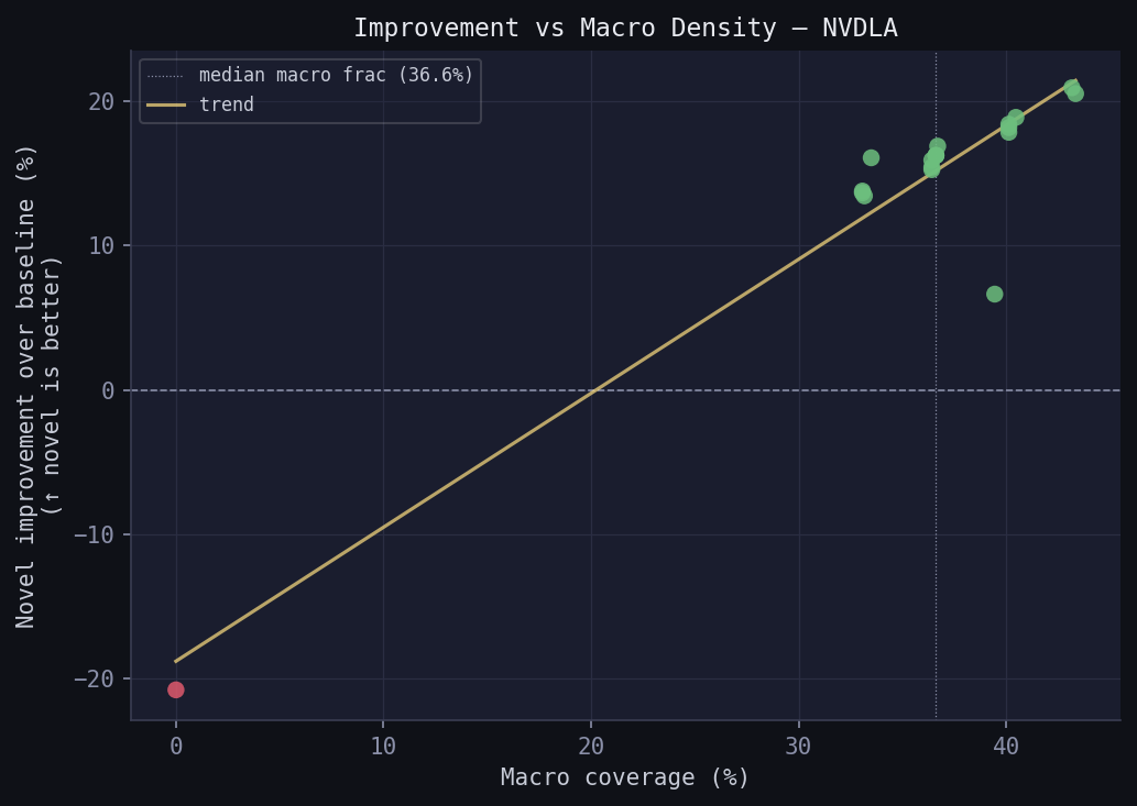
5. The improvement is consistent across samples, not driven by outliers. On NVDLA, novel wins on 18/19 val samples (94.7%). The per-sample scatter (fig_D) shows almost all points below the parity line regardless of macro density, confirming the gain is structural.
6. The recommended config is 5ch+corrected, not 6ch. Best MSE (0.00185), best SSIM (0.4028), best boundary MSE (0.00205) on synthetic ablation. No correlation penalty. On real data where n=96, 6ch still wins overall — but the ablation on controlled synthetic data makes clear that rudy_corrected is doing the work and macro_halo adds noise at small n.
Setup
git clone https://github.com/Mummanajagadeesh/pd-congestion-ml
cd pd-congestion-ml
pip install -r requirements.txt
Generate synthetic data
python3 data/gen_synthetic.py --n_samples 200
Train (synthetic)
python3 train.py --epochs 30 --batch_size 8
Train (real data — requires CircuitNet-N14 download)
# Download Vortex-small or NVDLA-small from CircuitNet-N14
# Extract to data/Vortex-small/ or data/nvdla-small/
python3 data/prepare_real.py   # for Vortex-small → data/real/
# modify REAL_BASE in prepare_real.py for other designs

python3 train.py --epochs 50 --batch_size 8 \
  --dataroot data/real_nvdla \
  --save_dir checkpoints/nvdla_50ep
Run real data study (Experiments A–E)
python3 analysis/real_data_study.py
# outputs: analysis/real_data_study.json + analysis/figures/fig_[A-E]_*.png
Evaluate and analyze
python3 eval.py
python3 analysis/region_error_breakdown.py
python3 analysis/ablation.py
python3 analysis/macro_sensitivity.py
python3 analysis/visualize.py
python3 analysis/generate_all_figures.py   # regenerate all figures from saved JSONs
python3 analysis/summary.py               # print all results from saved JSONs
Limitations
The real-data SSIM values (0.03–0.06) are low across all models. Two reasons: 96 samples is small for a real chip dataset, and the 128×128 resize from 459×456 or 809×802 loses spatial detail. The CircuitNet paper reports SSIM ~0.89 on their full N14 dataset with 10,000+ samples and 256×256 resolution. Our numbers are not comparable — they’re from a 96-sample subset used to validate the feature engineering direction, not to claim state-of-the-art.
The macro correction applied to real data works on precomputed RUDY maps (zero interior, redistribute to perimeter) rather than raw net lists. This is an approximation — the ideal correction would recompute RUDY from DEF with macro-aware routing, which requires running the full feature extraction pipeline with LEF/DEF files.
References
- CircuitNet — dataset and baselines
- RUDY — Zhong et al., DAC 2015 — original RUDY formulation
- ST-FPN — CircuitNet 2.0 paper
- RouteNet — Xie et al., ICCAD 2018