
Branch Pred. and Cache Replacement Eval ML Tool
ulearn-arch
ML-based branch prediction and cache replacement evaluation on ChampSim simulation traces.
Background
Hardware branch predictors (bimodal, gshare, TAGE) and cache replacement policies (LRU, RRIP) operate under strict area and latency budgets — typically 1–2 cycle prediction latency, kilobytes of storage. ML models don’t have those constraints offline. The question is: given full observability of branch history and cache access patterns, how much can ML improve over hardware baselines, and where does it fail?
This project instruments ChampSim — the standard simulator used in branch prediction (CBP) and cache replacement (CRC) championships — with custom logging modules, generates both synthetic and real program traces, and trains ML models on the resulting data.
Repo Structure
ulearn-arch/
├── champsim/                        # ChampSim submodule (instrumented)
│   ├── branch/
│   │   └── branch_logger/           # Bimodal + CSV logger for every branch decision
│   └── replacement/
│       └── cache_logger/            # LRU + CSV logger for every LLC eviction/fill
├── tracer/
│   └── gen_trace.py                 # Synthetic trace generator (5 patterns + mixed)
├── branch/
│   ├── train.py                     # v1: global history + PC features
│   └── train_v2.py                  # v2: adds per-PC local history
├── cache/
│   └── train.py                     # Within-set victim prediction
├── analysis/
│   ├── ipc_table.py                 # Extract IPC/MPKI from ChampSim JSON
│   ├── ipc_projection.py            # Project IPC gain from MPKI reduction
│   └── real_trace_analysis.py       # Branch bias analysis on real traces
└── data/                            # Traces and CSV logs (gitignored)
How It Works
Step 1 — Trace Generation
We generate synthetic ChampSim traces in the correct input_instr binary format. Each instruction is 64 bytes encoding: IP, branch flag, branch taken, source/destination registers, and memory addresses.
Branch type is inferred by ChampSim from register usage — BRANCH_CONDITIONAL requires:
dst_registerscontainsREG_IP(26)src_registerscontainsREG_IP(26) andREG_FLAGS(25)
We support 5 pure patterns plus a realistic mixed workload:
| Pattern | Description |
|---|---|
always_taken |
Every branch taken |
never_taken |
No branch taken |
alternating |
T, NT, T, NT, … |
random |
Coin-flip per branch |
loop |
Taken 7×, not-taken 1× (loop-of-8) |
mixed |
5 concurrent “functions” with different patterns + phase switching |
Real traces are collected using Intel PIN with ChampSim’s bundled tracer (champsim/tracer/pin/), tracing actual Linux programs (ls, sort).
Step 2 — ChampSim Instrumentation
Branch Logger (champsim/branch/branch_logger/) replaces the bimodal predictor. It maintains the same 2-bit saturating counter table but hooks into predict_branch() and last_branch_result() to log:
pc, global_history, prediction, actual, branch_type
global_history is a 16-bit shift register updated on every branch outcome. This gives the ML models the same global history that hardware perceptron predictors use.
Cache Logger (champsim/replacement/cache_logger/) replaces LRU in the LLC. It logs every eviction and fill event with:
set, way, full_addr, ip, victim_addr, access_count, fill_count,
lru_age, reuse_distance, is_dirty, is_prefetch, access_type, event
reuse_distance was added in v2 of the logger — cycles since this way was last accessed, an approximation of stack distance.
Step 3 — ML Training
For branch prediction (v1), we extract 17 features per branch: 16 bits of global history unpacked as individual binary features + PC lower bits. We compare Perceptron, Decision Tree, and Random Forest against bimodal.
For branch prediction (v2), we add 8 bits of per-PC local history (independent shift register per PC) + an additional PC hash field, giving 26 features total. This was added after v1 failed on real traces.
For cache replacement, we frame it as binary classification: at each eviction, compare the victim way against a sampled non-victim way from the same set, using access_count and fill_count. lru_age and reuse_distance are excluded — they directly encode recency and trivially separate the classes.
Setup & Usage
1. Clone and build ChampSim
git clone https://github.com/Mummanajagadeesh/ulearn-arch
cd ulearn-arch
git submodule update --init --recursive

cd champsim
vcpkg/bootstrap-vcpkg.sh
vcpkg/vcpkg install

# Copy headers to where ChampSim expects them
mkdir -p vcpkg/installed/x64-linux/include
cp -r vcpkg/packages/fmt_x64-linux/include/*          vcpkg/installed/x64-linux/include/
cp -r vcpkg/packages/cli11_x64-linux/include/*         vcpkg/installed/x64-linux/include/
cp -r vcpkg/packages/nlohmann-json_x64-linux/include/* vcpkg/installed/x64-linux/include/
cp -r vcpkg/packages/catch2_x64-linux/include/*        vcpkg/installed/x64-linux/include/
cp -r vcpkg/packages/bzip2_x64-linux/include/*         vcpkg/installed/x64-linux/include/
cp -r vcpkg/packages/liblzma_x64-linux/include/*       vcpkg/installed/x64-linux/include/

./config.sh champsim_config.json
make -j$(nproc)
cd ..
2. Install Python dependencies
pip install pandas scikit-learn matplotlib
3. Generate traces
mkdir -p data

for pattern in always_taken never_taken alternating random loop; do
    python3 tracer/gen_trace.py --instrs 1000000 --pattern $pattern \
        --out data/${pattern}.champsimtrace.xz
done

# Mixed trace
python3 - << 'EOF'
import importlib.util, lzma
spec = importlib.util.spec_from_file_location("gen_trace", "tracer/gen_trace.py")
m = importlib.util.module_from_spec(spec)
spec.loader.exec_module(m)
data = m.gen_mixed_trace(1_000_000)
with lzma.open('data/mixed.champsimtrace.xz', 'wb') as f:
    f.write(data)
EOF
4. Generate real traces (requires Intel PIN)
cd champsim/tracer/pin
make PIN_ROOT=/path/to/pin
cd ../../..

/path/to/pin/pin -t champsim/tracer/pin/obj-intel64/champsim_tracer.so \
    -o data/sort_real.champsimtrace -s 0 -t 1000000 \
    -- sort /usr/share/dict/words > /dev/null
xz -T0 data/sort_real.champsimtrace
5. Run ChampSim and collect traces
for pattern in always_taken never_taken alternating random loop mixed; do
    ./champsim/bin/champsim \
        --warmup-instructions 200000 \
        --simulation-instructions 500000 \
        --json data/stats_${pattern}.json \
        data/${pattern}.champsimtrace.xz
    mv branch_trace.csv data/branch_trace_${pattern}.csv
    mv cache_trace.csv  data/cache_trace_${pattern}.csv
done
6. Train and evaluate
python3 branch/train.py        # v1
python3 branch/train_v2.py     # v2 with local history
python3 cache/train.py
python3 analysis/ipc_table.py
python3 analysis/ipc_projection.py
python3 analysis/real_trace_analysis.py
Results
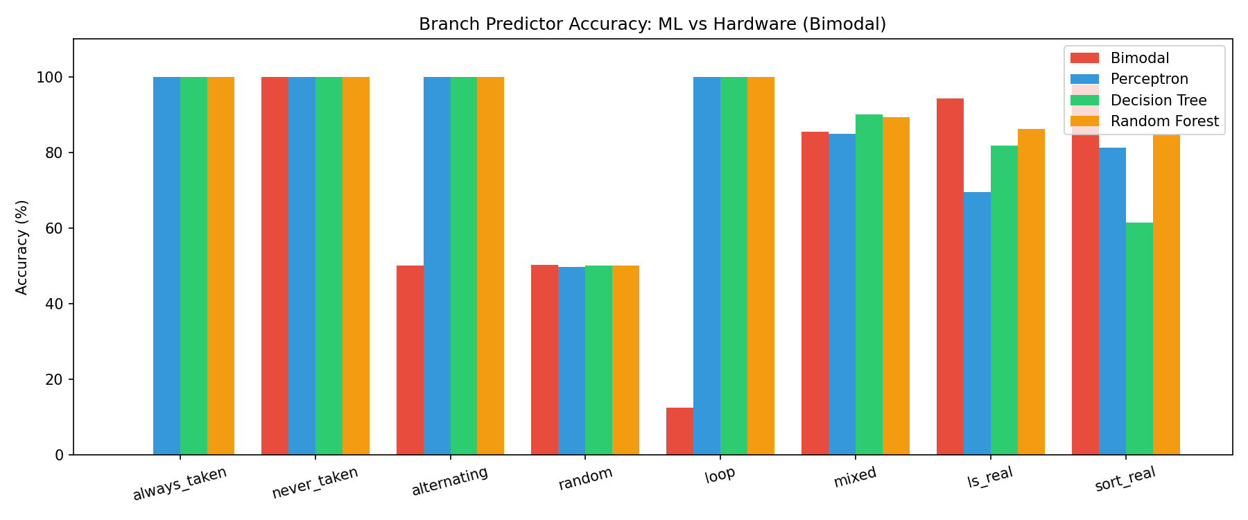
Branch Prediction — Pure Patterns
| Pattern | Bimodal | Perceptron | Decision Tree | Random Forest |
|---|---|---|---|---|
| always_taken | 0.0% | 100% | 100% | 100% |
| never_taken | 100% | 100% | 100% | 100% |
| alternating | 50.0% | 100% | 100% | 100% |
| random | 50.3% | 49.7% | 50.0% | 50.4% |
| loop (8-cycle) | 12.5% | 100% | 100% | 100% |
Why bimodal fails on loop:
The loop-of-8 pattern takes 7 times then doesn’t take once. Bimodal’s 2-bit saturating counter stabilizes to “strongly taken” and never recovers in time for the single not-taken exit. It mispredicts the loop exit every single iteration — 12.5% accuracy means it’s correct only on the 1 non-branch instruction out of 8.
Why ML gets loop right:
Global history captures the last 16 branch outcomes as a binary vector. After seeing 1111111 in history, the next outcome is always 0. A decision tree learns this split in a single node. Perceptron learns the weight pattern. Both achieve 100%.
Why alternating fools bimodal:
The 2-bit counter oscillates between states 01 and 10 (weakly not-taken / weakly taken), predicting wrong every other branch — stuck at 50%. ML sees the alternating 0,1,0,1 in history bits and learns the parity in one split.
Why random is 50% for everyone:
Genuinely unpredictable. No feature — history, PC, or any combination — predicts a coin flip. This is the theoretical floor and confirms models aren’t overfitting.
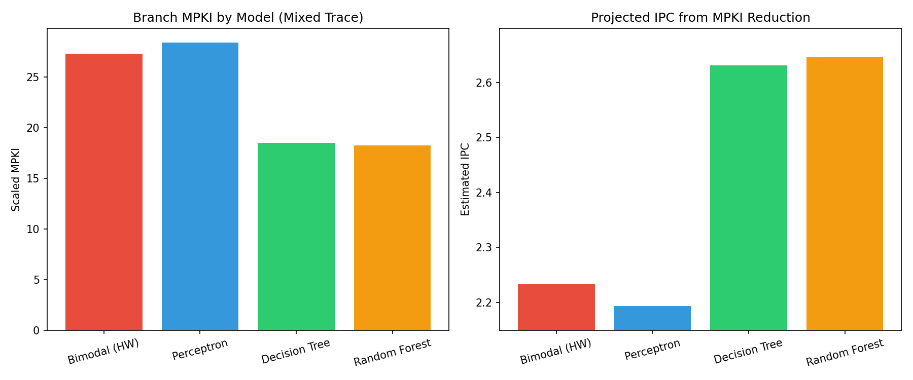
Branch Prediction — Mixed Workload
| Model | Accuracy | MPKI | Δ vs Bimodal |
|---|---|---|---|
| Bimodal (hardware) | 85.38% | 146.2 | baseline |
| Perceptron | 84.81% | 151.9 | −0.57%, +5.7 MPKI |
| Decision Tree | 90.09% | 99.1 | +4.71%, −47.1 MPKI |
| Random Forest | 90.24% | 97.6 | +4.86%, −48.6 MPKI |
The mixed trace combines 5 concurrent branch behaviors (loop-8, loop-16, alternating, random, biased-90%) with phase switching every 10,000 instructions. Bimodal’s global table sees aliasing between PCs across different phases, causing interference. ML models with PC as an explicit feature can condition predictions on which “function” they’re in, reducing aliasing.
Perceptron performs worse than bimodal here. Phase-switching behavior requires non-linear decision boundaries that a linear model can’t learn. This mirrors real hardware results where hashed perceptrons outperform plain perceptrons by handling aliasing better.
IPC Projection (Mixed Trace)
Using ROB occupancy at mispredict (7.697 cycles) from ChampSim JSON. Base IPC = 2.2331.
| Model | Est. IPC | Δ IPC | Δ % |
|---|---|---|---|
| Bimodal | 2.2331 | — | — |
| Perceptron | 2.1929 | −0.040 | −1.8% |
| Decision Tree | 2.6312 | +0.398 | +17.8% |
| Random Forest | 2.6458 | +0.413 | +18.5% |
Cache Replacement
| Model | Accuracy | vs Baseline |
|---|---|---|
| Majority class baseline | 50.0% | — |
| Logistic Regression | 70.3% | +20.3% |
| Decision Tree | 70.3% | +20.3% |
| Random Forest | 70.3% | +20.3% |
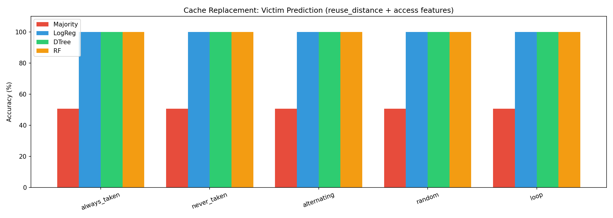
Task framing (corrected from earlier version):
At each eviction, compare the victim way against a randomly sampled non-victim way from the same set, using access_count and fill_count as features. This is the correct within-set formulation — we’re asking whether these features alone can identify which way is the LRU victim, without using any recency signal directly.
Top feature: fill_count
Ways that have been replaced more times are evicted again sooner. High fill_count indicates a hot conflict set slot. All models converge on a threshold split on this feature.
Why all models plateau at 70.3%:
fill_count threshold is the only learnable boundary with these two features. The remaining ~30% is structural — LRU ordering within a set depends on the exact access sequence which fill_count and access_count alone can’t fully reconstruct.
Note: real traces (ls_real, sort_real) had zero LLC evictions — working sets fit entirely in the 2048-set × 16-way LLC for short trace segments.
Branch Prediction — Real Traces (PIN-traced ls, sort)
v1: global history + PC features only
| Trace | Bimodal | Perceptron | Decision Tree | Random Forest |
|---|---|---|---|---|
| ls (85k branches, 1995 PCs) | 94.23% | 69.54% | 81.79% | 86.08% |
| sort (84k branches, 2170 PCs) | 97.85% | 81.28% | 61.45% | 84.86% |
ML loses to bimodal on both. 84–85% of branch PCs in real programs are highly biased (>95% always-taken or always-not-taken). Bimodal converges on these quickly. Global history from other PCs adds noise for biased branches — actively hurts.
ls_real:   1677/1995 PCs (84.1%) are >95% biased in one direction
sort_real: 1843/2170 PCs (84.9%) are >95% biased in one direction
Only 6-7% of PCs have hard branches (30-70% taken rate)
v2: global history + per-PC local history (8-bit shift register per PC)
| Trace | Bimodal | RF global-only | RF global+local | GBDT global+local |
|---|---|---|---|---|
| mixed | 85.38% | 90.68% (+5.30%) | 90.47% (+5.09%) | 90.51% (+5.13%) |
| ls_real | 96.97% | 76.62% (−20.35%) | 97.12% (+0.15%) | 96.71% (−0.26%) |
| sort_real | 99.82% | 99.93% (+0.11%) | 99.93% (+0.11%) | 99.87% (+0.04%) |
Adding 8 bits of per-PC local history closes the gap on ls_real: RF goes from −20.35% to +0.15% vs bimodal. The −20% for global-only is not a small degradation — global history from other PCs contaminates predictions when it dominates the history register, making it worse than a counter that just remembers what this PC did last.
sort_real is already 99.82% with bimodal — essentially no room to improve, all models converge.
This is the feature engineering insight behind TAGE: per-PC tagged history tables of multiple lengths. Global-only approaches are actively harmful for real workloads compared to per-PC history.
IPC Summary (from ChampSim JSON)
| Pattern | IPC | Branch MPKI | LLC MPKI |
|---|---|---|---|
| always_taken | 0.2163 | 199.95 | 62.47 |
| never_taken | 0.2167 | 0.00 | 62.47 |
| alternating | 0.2159 | 99.92 | 62.47 |
| random | 0.2169 | 137.42 | 62.47 |
| loop | 0.2159 | 199.84 | 62.47 |
| mixed | 2.2331 | 27.30 | 0.00 |
Pure synthetic patterns are memory-bound (LLC MPKI ~62), so branch misprediction impact on IPC is masked by LLC miss latency — IPC stays ~0.216 regardless of branch accuracy. The mixed trace fits in cache (LLC MPKI=0), so branch prediction is the bottleneck — IPC 2.23 with bimodal, projected 2.65 with Random Forest.
Notes on Framing
The offline ML setting here differs from hardware deployment. These models have access to full global history, per-PC local history, and exact PC values — hardware predictors approximate this with kilobytes of storage. The accuracy numbers are not directly comparable to hardware accuracy under area constraints.
The v1 vs v2 gap on real traces (−20% to +0.15% by adding local history) shows that per-PC history is not optional for real workloads — using global history alone on real programs is actively harmful compared to bimodal. The gap where ML has measurable advantages is in structured non-biased branches: loops, phase-switching code, correlated branch sequences.