Model Design, Training, and Quantization
CIFAR-10 CNN — Model Design, Training, and Quantization
This document covers the full model development pipeline: dataset characteristics, training setup, architectural exploration across eight model variants, and fixed-point quantization evaluation for hardware deployment. All models are trained on CIFAR-10 and evaluated for both software accuracy and hardware suitability on resource-constrained FPGAs.
Dataset: CIFAR-10
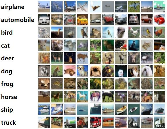
CIFAR-10 consists of 60,000 color images across 10 classes, with 6,000 images per class. The training split contains 50,000 images and the test split contains 10,000 images. Each image is 32×32 pixels with three color channels (RGB).
The ten classes and their visual characteristics:
| Class | Description |
|---|---|
| Airplane | Various orientations and backgrounds, full aircraft visible |
| Automobile | Cars and vehicles, typically side or front view |
| Bird | Various species, perched or in flight |
| Cat | Domestic cats, diverse postures and backgrounds |
| Deer | Natural settings, standing or grazing |
| Dog | Various breeds and poses |
| Frog | Natural environments, often on plants or water |
| Horse | Different stances, fields or riding contexts |
| Ship | Watercraft on water bodies |
| Truck | On roads or in industrial settings |
The images are small, low-resolution, and contain varied backgrounds, making CIFAR-10 challenging despite its simplicity. The limited resolution means models must learn compact, discriminative features rather than relying on fine detail. The visual similarity between classes such as cat/dog and automobile/truck introduces additional difficulty — this shows up consistently in the confusion patterns across all implementations in this project.
Training Setup
All models are trained end-to-end on Google Colab with GPU acceleration. Training is implemented in TensorFlow/Keras.
Data Augmentation
Extensive augmentation is applied to the training set to reduce overfitting and improve generalization. The model sees varied versions of each image during training, which encourages robustness to small input perturbations:
from tensorflow.keras.preprocessing.image import ImageDataGenerator

datagen = ImageDataGenerator(
    rotation_range=15,
    horizontal_flip=True,
    width_shift_range=0.1,
    height_shift_range=0.1,
)
datagen.fit(x_train)
Augmentations applied:
- Random rotation up to ±15°
- Horizontal flip (random left-right mirror)
- Width shift up to ±10% of image width
- Height shift up to ±10% of image height
Online augmentation is used — each batch is augmented on-the-fly during training rather than pre-generating an augmented dataset. This means the model effectively sees a different augmented version of each image every epoch, providing maximum diversity across 100 epochs.
Optimizer: Adam
All models are compiled with the Adam optimizer, which combines adaptive learning rates with momentum. Given parameters θ at step t:
m_t = β₁·m_{t-1} + (1−β₁)·∇L(θ_{t-1})          # first moment (mean)
v_t = β₂·v_{t-1} + (1−β₂)·(∇L(θ_{t-1}))²        # second moment (variance)
m̂_t = m_t / (1−β₁ᵗ)                              # bias-corrected mean
v̂_t = v_t / (1−β₂ᵗ)                              # bias-corrected variance
θ_t = θ_{t-1} − α · m̂_t / (√v̂_t + ε)            # parameter update
where β₁ and β₂ are decay rates, α is the learning rate, and ε prevents division by zero. Adam’s adaptive per-parameter learning rates accelerate convergence for deeper networks compared to fixed-rate SGD, and the momentum term smooths noisy gradient updates.
Loss Function: Categorical Cross-Entropy
Standard multi-class classification loss. For true label vector y and predicted probabilities ŷ over C = 10 classes:
L(y, ŷ) = −Σᵢ yᵢ · log(ŷᵢ)
One-hot encoded labels are used — yᵢ = 1 for the correct class, 0 for all others. The loss penalizes confident wrong predictions heavily via the log term.
model.compile(
    optimizer='adam',
    loss='categorical_crossentropy',
    metrics=['accuracy']
)
Training Configuration
| Parameter | Value |
|---|---|
| Batch size | 64 |
| Max epochs | 100 |
| Input | Augmented via datagen.flow() |
| Validation | Full test set (10,000 images) |
history = model.fit(
    datagen.flow(x_train, y_train, batch_size=64),
    validation_data=(x_test, y_test),
    epochs=100,
    callbacks=[lr_reduction, early_stop],
    verbose=1
)
Learning Rate Scheduling and Early Stopping
Two callbacks control the training dynamics:
ReduceLROnPlateau monitors validation accuracy and halves the learning rate if it does not improve for 5 consecutive epochs. This allows the optimizer to make finer weight adjustments as it approaches a minimum — large learning rates are useful early in training for fast convergence, but smaller rates are needed later to settle precisely.
EarlyStopping halts training if validation accuracy does not improve for 15 epochs and restores the best weights seen during training. This prevents unnecessary computation and avoids overfitting to the training set after the model has already converged.
from tensorflow.keras.callbacks import ReduceLROnPlateau, EarlyStopping

lr_reduction = ReduceLROnPlateau(
    monitor='val_accuracy', patience=5, factor=0.5, verbose=1
)
early_stop = EarlyStopping(
    monitor='val_accuracy', patience=15, restore_best_weights=True
)
Architectural Exploration
Eight architectures were explored in sequence. Each step was motivated by the constraints of the target hardware — progressively reducing parameters, FLOPs, and architectural complexity while tracking the accuracy penalty of each simplification.
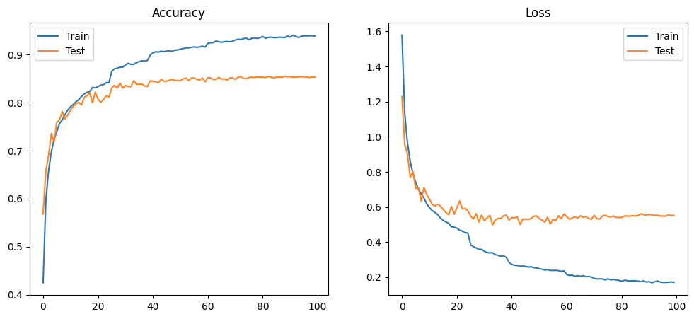
MODEL_ARCH_1 — Deep CNN Baseline
Three convolutional blocks with 64→128→256 filters, Batch Normalization (BN) after each block, ReLU activations, and a Dense(512) fully connected layer before the softmax classifier.
BN normalizes intermediate activations to zero mean and unit variance, reducing internal covariate shift and enabling higher stable learning rates. This stabilization is the primary reason ARCH_1 achieves the highest accuracy of the series. The Dense(512) layer provides substantial representational capacity before classification.
90.91% accuracy, 3,253,834 parameters, 276.5M FLOPs. Far too large for any of the target FPGA devices.
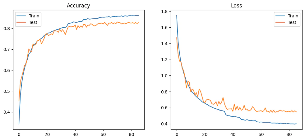
MODEL_ARCH_2 — Reduced Filters
Filter sizes reduced to 32→64→128, Dense layer reduced to Dense(256), BN
retained. The reduction in filter count at each layer is the primary driver
of the parameter reduction — each convolutional layer’s parameter count scales
with input_channels × output_channels × kernel_size².
88.84% accuracy, 816,938 parameters, 99.7M FLOPs. Still substantially smaller than ARCH_1 but still impractical for small Zynq devices.
MODEL_ARCH_3 — Batch Normalization Removed
BN removed entirely from ARCH_2 (96 filters in final block). This simplifies inference hardware significantly — BN requires storing running mean and variance per channel and computing a normalization at each layer output, which adds hardware logic and memory. Without BN, every layer is a pure convolution + activation, directly implementable as MAC + ReLU.
85.53% accuracy, 517,002 parameters, 68.2M FLOPs. The accuracy drop from removing BN (88.84% → 85.53%) is the cost of this hardware simplification.
MODEL_ARCH_4 — Global Average Pooling Replaces Dense
The Dense(256) layer replaced by Global Average Pooling (GAP). GAP averages each feature map spatially, producing one value per channel before the final Dense(10) classifier. This eliminates the large matrix multiply of the fully connected layer.
The parameter count drop from ARCH_3 to ARCH_4 is dramatic: 517k → 72.7k. Almost all of those parameters were in the Dense layer — the convolutional layers have relatively few parameters. GAP also acts as a regularizer: because each output directly represents a channel average, the model cannot memorize spatial patterns in the final activation map.
83.05% accuracy, 72,730 parameters, 20.4M FLOPs. This is the turning point where the model becomes feasible for small FPGA devices.
MODEL_ARCH_5 — Minimal Two-Block Network
Reduced to only two convolutional blocks with 16→32 filters and GAP. This is the smallest practical architecture tested.
67.94% accuracy, 16,986 parameters, 7.2M FLOPs. The accuracy collapse (83% → 68%) shows the representational capacity floor — 16→32 filters is insufficient to learn discriminative features for 10-class CIFAR-10.
MODEL_ARCH_6 — Filter Count Recovered
ARCH_5 structure kept, filter count increased to 32→64. This recovers representational capacity lost in ARCH_5 without adding structural complexity.
78.92% accuracy, 66,218 parameters, 13.8M FLOPs. The 11-point accuracy recovery (67.94% → 78.92%) with only a 4× parameter increase confirms that filter count, not depth, was the binding constraint in ARCH_5.
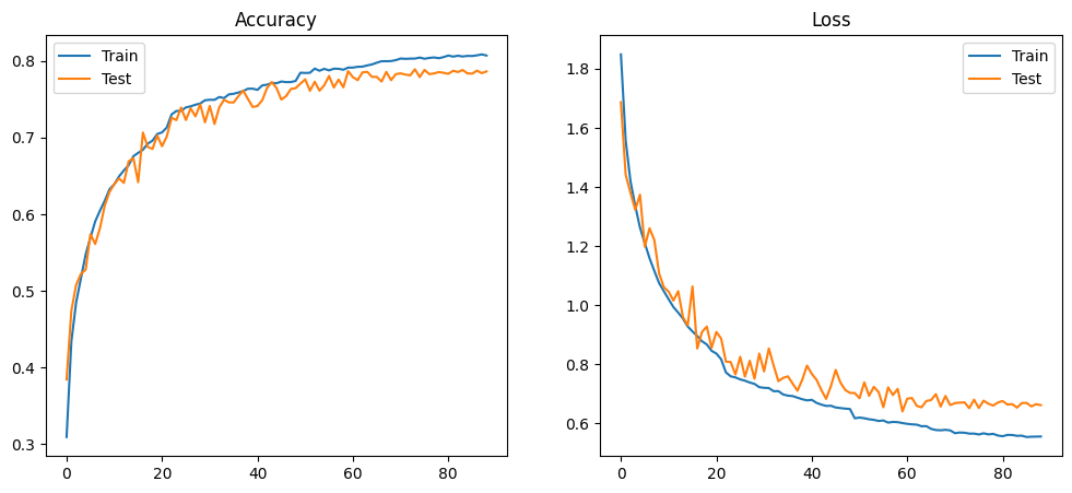
MODEL_ARCH_7 — Residual Connections Introduced
Residual (skip) connections added to ARCH_6’s two-block structure. Each convolutional block receives a 1×1 convolutional shortcut that matches the output channel count. The shortcut allows gradients to flow directly to earlier layers during backpropagation, mitigating vanishing gradient issues and enabling better feature reuse.
The 1×1 shortcut convolution: when input and output channel counts differ (e.g., 3→32 at Block 1), a 1×1 conv is applied to the input to project it to the correct number of channels before addition. This is the same structure used throughout the hardware implementations.
81.08% accuracy, 68,458 parameters, 15.2M FLOPs. The 2-point gain over ARCH_6 (78.92% → 81.08%) at comparable parameter count demonstrates the accuracy benefit of residual connections.
MODEL_ARCH_8 — Reduced Filter Residual Network (Final)
ARCH_7 structure with filter counts reduced to 28→56. This fine-tunes the balance between representational capacity and hardware resource usage. 28 and 56 were chosen to fit within the BRAM and DSP budgets of the target devices (xc7z010, xc7z020).
80.45% accuracy, 52,622 parameters, 12.6M FLOPs. This is the architecture used in all hardware implementations — manual HLS, hls4ml, FINN/Brevitas, and RTL Verilog.
Architecture Summary
| Model | Key Structure | Accuracy | Parameters | FLOPs (M) |
|---|---|---|---|---|
| ARCH_1 | 64→128→256, BN, Dense512 | 90.91% | 3,253,834 | 276.5 |
| ARCH_2 | 32→64→128, BN, Dense256 | 88.84% | 816,938 | 99.7 |
| ARCH_3 | 32→64→96, no BN, Dense256 | 85.53% | 517,002 | 68.2 |
| ARCH_4 | 16→32→64, GAP, Dense10 | 83.05% | 72,730 | 20.4 |
| ARCH_5 | 16→32, GAP, Dense10 | 67.94% | 16,986 | 7.2 |
| ARCH_6 | 32→64, GAP, Dense10 | 78.92% | 66,218 | 13.8 |
| ARCH_7 | Residual 32→64 + 1×1 shortcuts, GAP | 81.08% | 68,458 | 15.2 |
| ARCH_8 | Residual 28→56 + 1×1 shortcuts, GAP | 80.45% | 52,622 | 12.6 |
Here’s the FOM calculated for all 8 architectures, then the markdown section:
FOM = Accuracy / √(Params × FLOPs×10⁶)
| Model | Accuracy | Params | FLOPs (M) | √(P×F) | FOM (×10⁻⁵) |
|---|---|---|---|---|---|
| ARCH_1 | 90.91 | 3,253,834 | 276.5M | 30,023,580 | 3.03 |
| ARCH_2 | 88.84 | 816,938 | 99.7M | 9,026,834 | 9.84 |
| ARCH_3 | 85.53 | 517,002 | 68.2M | 5,939,778 | 14.40 |
| ARCH_4 | 83.05 | 72,730 | 20.4M | 1,218,732 | 68.14 |
| ARCH_5 | 67.94 | 16,986 | 7.2M | 349,641 | 194.3 |
| ARCH_6 | 78.92 | 66,218 | 13.8M | 956,010 | 82.55 |
| ARCH_7 | 81.08 | 68,458 | 15.2M | 1,020,594 | 79.44 |
| ARCH_8 | 80.45 | 52,622 | 12.6M | 814,466 | 98.78 |
ARCH_8 is the best among the serious candidates (ARCH_4 onwards). ARCH_5’s high FOM is misleading — 67.94% accuracy is practically unusable.
Hardware Efficiency: Figure of Merit
To compare architectures on a combined accuracy-vs-cost axis, the following figure of merit is used:
FOM = Accuracy / sqrt(Parameters x FLOPs)
This penalizes models that are expensive in either dimension: parameter count (memory, weight storage) or FLOPs (compute, latency). A higher FOM indicates better accuracy per unit of hardware cost. The target accuracy for this project is 80%, establishing a minimum threshold for hardware deployment candidates.
| Model | Accuracy | Parameters | FLOPs (M) | FOM (×10⁻⁵) |
|---|---|---|---|---|
| ARCH_1 | 90.91% | 3,253,834 | 276.5 | 3.03 |
| ARCH_2 | 88.84% | 816,938 | 99.7 | 9.84 |
| ARCH_3 | 85.53% | 517,002 | 68.2 | 14.40 |
| ARCH_4 | 83.05% | 72,730 | 20.4 | 68.14 |
| ARCH_5 | 67.94% | 16,986 | 7.2 | 194.3 |
| ARCH_6 | 78.92% | 66,218 | 13.8 | 82.55 |
| ARCH_7 | 81.08% | 68,458 | 15.2 | 79.44 |
| ARCH_8 | 80.45% | 52,622 | 12.6 | 98.78 |
ARCH_5 has the highest raw FOM but its 67.94% accuracy falls below the minimum useful threshold for CIFAR-10 classification. Among architectures with acceptable accuracy (above 78%), ARCH_8 has the best FOM. The residual connections recover accuracy at no additional parameter cost relative to ARCH_6, pushing its efficiency above ARCH_6 and ARCH_7 despite the reduced filter count from ARCH_7.
Training and Loss Curves
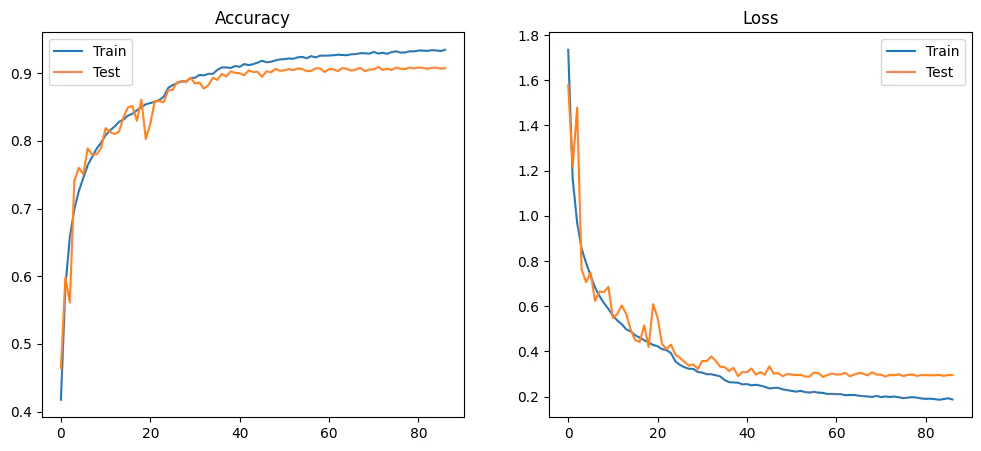 MODEL_ARCH_1 — 90.91%
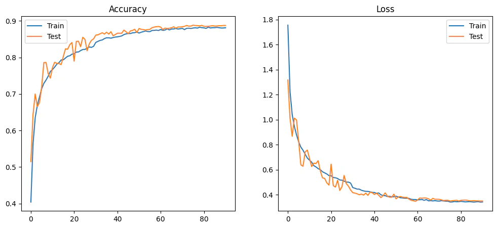 MODEL_ARCH_2 — 88.84%
 MODEL_ARCH_3 — 85.53%
 MODEL_ARCH_4 — 83.05%
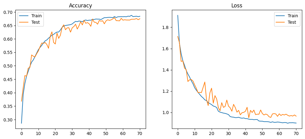 MODEL_ARCH_5 — 67.94%
 MODEL_ARCH_6 — 78.92%
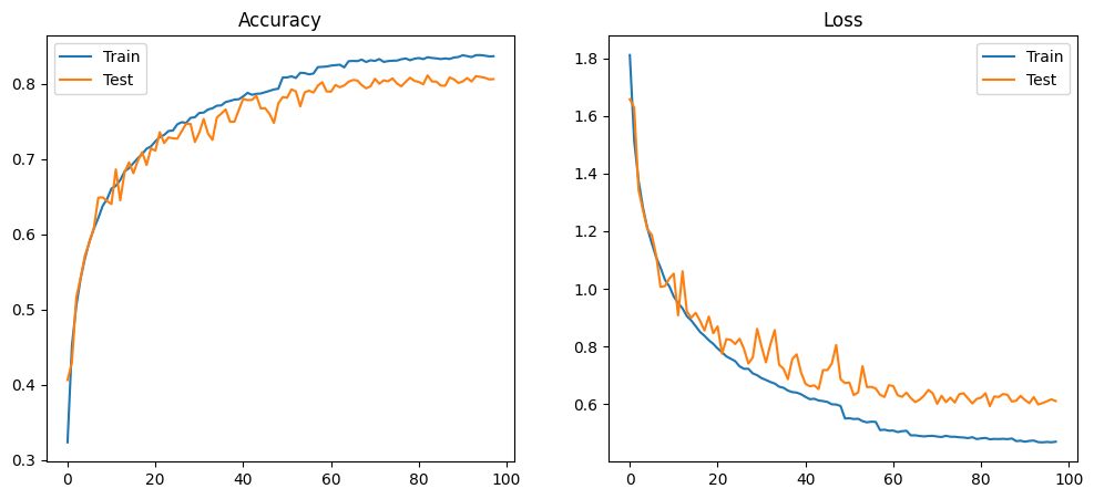 MODEL_ARCH_7 — 81.08%
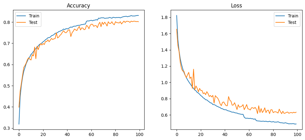 MODEL_ARCH_8 — 80.45%
Model Quantization
Why Quantize
Floating-point arithmetic — FP32 in particular — is expensive in hardware. FP32 multipliers occupy significant LUT and DSP area on FPGAs and consume considerable power. For a model with 52,622 parameters at FP32, every weight requires a 32-bit floating-point multiplier in the MAC datapath. By reducing weights and activations to fixed-point integers, simpler and smaller arithmetic units can be used, memory footprint decreases, parallelism increases, and power consumption drops — all critical for edge FPGA deployment.
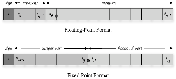
Floating-Point vs Fixed-Point
Floating-point (FP32): 1 sign bit + 8 exponent bits + 23 mantissa bits. The exponent allows the value to scale over an enormous range, which is why FP32 is used for training — gradients and activations vary dramatically across layers and training steps. The hardware cost is high: FP32 multipliers require DSP blocks and significant routing.
Fixed-point (Qm.n): The decimal point is fixed at a predetermined position. No exponent — scaling is implicit. Arithmetic reduces to integer addition and multiplication, which FPGAs implement efficiently in LUT logic or DSP slices. The cost is reduced dynamic range: values outside the representable range overflow.
Concrete example for 0.625:
# FP8 (simplified floating-point, 8-bit)
0.625 → sign:0, exponent:011, mantissa:1010000

# Q1.7 fixed-point
0.625 × 2^7 = 80 → binary: 01010000
For neural network weights normalized to [-1, 1), fixed-point is sufficient because the dynamic range requirement is known and bounded.
Qm.n Fixed-Point Format
The Qm.n notation specifies:
- m — number of integer bits including the sign bit
- n — number of fractional bits
- Total width — m + n bits
The MSB is always the sign bit. The remaining m−1 bits are the integer magnitude. The n LSBs are the fractional part.
Representable range: [−2^(m−1), 2^(m−1) − 2^(−n)]
Step size (resolution): 2^(−n)
| Format | Total bits | Integer bits | Fractional bits | Range | Step |
|---|---|---|---|---|---|
| Q1.7 | 8 | 1 | 7 | [−1, 0.992] | 0.0078 |
| Q2.6 | 8 | 2 | 6 | [−2, 1.984] | 0.0156 |
| Q1.15 | 16 | 1 | 15 | [−1, 0.99997] | 0.00003 |
| Q4.12 | 16 | 4 | 12 | [−8, 7.9998] | 0.000244 |
Q1.7 is used throughout this project. With weights normalized to [-1, 1), m=1 is sufficient to cover the range without overflow. n=7 gives 128 discrete steps over [−1, 1), providing enough precision for inference without requiring larger multipliers.
Hardware Implications of Qm.n Choice
Integer bits (m): Too few causes overflow during accumulation, especially in deep layers where many MACs are summed. Too many increases multiplier bit-width unnecessarily, consuming more LUTs and DSPs.
Fractional bits (n): More bits reduce quantization error and preserve accuracy, but require wider multipliers. An 8-bit Q1.7 multiplier fits in a single DSP48 slice on Zynq. Doubling to Q1.15 doubles multiplier size.
Memory: Total bit-width directly determines weight storage. Reducing from FP32 (32 bits) to Q1.7 (8 bits) gives a 4× reduction in weight memory — from 291 KB to 72.7 KB for ARCH_4, and from 210 KB to 52.6 KB for ARCH_8.
Accumulation: When summing N fixed-point products, the accumulator must be wide enough to prevent overflow. For Q1.7 × Q1.7 = Q2.14, summing 504 such products (3×3 kernel × 56 channels) requires log₂(504) ≈ 9 additional bits. Accumulators in this project use 32-bit width throughout.
Latency and power: Narrower operands reduce switching activity and gate count, decreasing both latency and dynamic power. For battery-powered or thermally-constrained edge systems, this is the primary motivation for quantization beyond the memory savings.
Types of Quantization
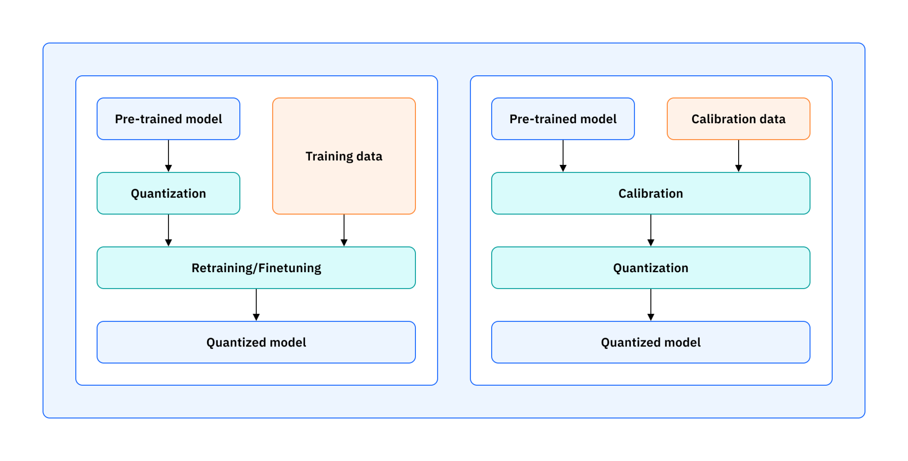
Post-Training Quantization (PTQ)
Converts a pre-trained float model to fixed-point after training without modifying the training process. Simple and fast — no retraining required. The accuracy loss comes from rounding trained float weights to the nearest representable fixed-point value.
import torch
from torch.quantization import quantize_dynamic

model_fp = MyModel()
model_int8 = quantize_dynamic(model_fp, {torch.nn.Linear}, dtype=torch.qint8)
For a weight w_fp, the PTQ conversion is:
w_q = round(w_fp × (2^n − 1))
PTQ is used in this project: float weights from Keras training are converted to
Q1.7 integers using the fixed.py / fixed_hdshk.py scripts across all RTL
and C implementations.
Tradeoff: Fast, no retraining, small accuracy loss — acceptable when the model is already trained and the quantization error is within tolerable limits.
Quantization-Aware Training (QAT)
Simulates quantization during training by inserting fake quantization nodes in the forward pass. These nodes apply rounding and truncation to simulate fixed-point behavior, while gradients are computed using the Straight-Through Estimator (STE) — the gradient passes through the rounding operation as if it were the identity function, allowing normal backpropagation.
import torch
from torch.quantization import prepare_qat, convert

model_fp = MyModel()
model_fp.train()
model_qat = prepare_qat(model_fp)        # insert fake-quant nodes
train(model_qat, train_loader, epochs=5) # train with simulated quantization
model_int8 = convert(model_qat)          # convert to real quantized model
QAT is used in the Brevitas + FINN implementation. Brevitas applies QAT
during the PyTorch training phase using QuantConv2d and QuantReLU layers
that simulate 4-bit weight and activation quantization. The model learns
weights that are already robust to the rounding errors introduced by 4-bit
quantization, rather than having those errors imposed post-hoc.
Tradeoff: Higher accuracy at low bit-widths (especially 4-bit and below) at the cost of a retraining phase. QAT is necessary when PTQ accuracy loss is unacceptable — which is typically the case below 6–8 bits.
| PTQ | QAT | |
|---|---|---|
| Retraining required | No | Yes |
| Typical bit-width | ≥8 bits | 4–8 bits |
| Accuracy | Slight drop | Near-float |
| Complexity | Low | High |
| Used in this project | RTL, HLS, hls4ml, keras2c | Brevitas + FINN |
Quantization Evaluation on CIFAR-10
Both MODEL_ARCH_4 and MODEL_ARCH_8 were evaluated across multiple Qm.n formats using a 100-image test set (10 images per class). Python fixed-point simulation results are compared against Verilog hardware implementation results for each format.
Model size is computed as:
Model Size (bytes) = Number of Parameters × (Bit-width / 8)
MODEL_ARCH_4 (72,730 Parameters)
| Format | Accuracy | Model Size |
|---|---|---|
| Float32 | 85% | 291.0 KB |
| Q1.31 | 84% | 291.0 KB |
| Q1.15 | 84% | 145.0 KB |
| Q1.7 | 83% | 72.7 KB |
| Q1.3 | 65% | 36.4 KB |
Q1.31 and Q1.15 retain full accuracy (84–85%) with moderate to large memory savings. Q1.7 retains 83% accuracy at exactly 4× memory reduction from Float32 — a 1-point accuracy cost for a 4× memory saving. This is the operating point used in all hardware implementations. Q1.3 (4-bit total) drops to 65% — the fractional resolution is insufficient to represent weight variations accurately, causing widespread misclassification.
MODEL_ARCH_8 (52,622 Parameters)
| Format | Accuracy | Model Size |
|---|---|---|
| Float32 | 80% | 210.49 KB |
| Q1.31 | 84% | 210.49 KB |
| Q1.15 | 84% | 105.24 KB |
| Q1.7 | 83% | 52.62 KB |
| Q1.3 | 78% | 26.31 KB |
An interesting result: Q1.31 and Q1.15 outperform Float32 for ARCH_8 (84% vs 80%). This can occur when the training process leaves some noise in the float weights — rounding to fixed-point acts as implicit regularization, removing some of that noise. This is not guaranteed behavior but is a known phenomenon with small models where float weights have limited effective precision anyway.
Q1.7 again retains 83% with 4× memory reduction. Q1.3 drops less severely than in ARCH_4 (78% vs 65%) — ARCH_8’s residual connections provide more robust feature representations that are less sensitive to weight precision.
Quantization Summary
| Format | ARCH_4 Acc | ARCH_8 Acc | Bit reduction vs FP32 | Memory reduction |
|---|---|---|---|---|
| Float32 | 85% | 80% | 1× | 1× |
| Q1.31 | 84% | 84% | 1× | 1× |
| Q1.15 | 84% | 84% | 2× | 2× |
| Q1.7 | 83% | 83% | 4× | 4× |
| Q1.3 | 65% | 78% | 8× | 8× |
Q1.7 is the practical sweet spot for this project: 4× memory reduction,
minimal accuracy penalty (1–2%), and 8-bit arithmetic that maps directly to
DSP48 slices and LUT-based multipliers on Zynq FPGAs. Every hardware
implementation in this project — RTL Verilog, manual HLS, and the C/keras2c
implementations — uses Q1.7 weights. The hls4ml implementation uses
ap_fixed<16,6> (Q6.10 equivalent) and the Brevitas/FINN implementation uses
4-bit weights, both chosen for their respective toolchain constraints and target
device budgets.